s-jSDM
Scalable joint species distribution modeling

![]()
![]()
![]()
s-jSDM - Fast and accurate Joint Species Distribution Modeling
About the method
The method is described in Pichler & Hartig (2021) A new joint species distribution model for faster and more accurate inference of species associations from big community data, https://doi.org/10.1111/2041-210X.13687. The code for producing the results in this paper is available under the subfolder publications in this repo.
The method itself is wrapped into an R package, available under subfolder sjSDM. You can also use it stand-alone under Python (see instructions below). Note: for both the R and the python package, python >= 3.7 and pytorch must be installed (more details below).
Installing the R / Python package
R-package
Install the package via
install.packages("sjSDM")
Depencies for the package can be installed before or after installing the package. Detailed explanations of the dependencies are provided in vignette(“Dependencies”, package = “sjSDM”), source code here. Very briefly, the dependencies can be automatically installed from within R:
sjSDM::install_sjSDM(version = "gpu") # or
sjSDM::install_sjSDM(version = "cpu")
To cite sjSDM, please use the following citation:
citation("sjSDM")
Development
If you want to install the current (development) version from this repository, run
devtools::install_github("https://github.com/TheoreticalEcology/s-jSDM", subdir = "sjSDM", ref = "master")
Once the dependencies are installed, the following code should run:
Workflow
Simulate a community and fit a sjSDM model:
library(sjSDM)
## ── Attaching sjSDM ──────────────────────────────────────────────────── 1.0.4 ──

## ✔ torch <environment>
## ✔ torch_optimizer
## ✔ pyro
## ✔ madgrad
set.seed(42)
community <- simulate_SDM(sites = 100, species = 10, env = 3, se = TRUE)
Env <- community$env_weights
Occ <- community$response
SP <- matrix(rnorm(200, 0, 0.3), 100, 2) # spatial coordinates (no effect on species occurences)

model <- sjSDM(Y = Occ, env = linear(data = Env, formula = ~X1+X2+X3), spatial = linear(data = SP, formula = ~0+X1:X2), se = TRUE, family=binomial("probit"), sampling = 100L)
summary(model)
## Family:  binomial
##
## LogLik:  -510.9816
## Regularization loss:  0
##
## Species-species correlation matrix:
##
##  sp1  1.0000
##  sp2 -0.3780  1.0000
##  sp3 -0.2050 -0.4070  1.0000
##  sp4 -0.1850 -0.3860  0.8220  1.0000
##  sp5  0.6820 -0.4090 -0.1240 -0.0730  1.0000
##  sp6 -0.3050  0.4870  0.1630  0.1510 -0.1220  1.0000
##  sp7  0.5830 -0.1190  0.0960  0.1200  0.5520  0.2450  1.0000
##  sp8  0.3140  0.1690 -0.5280 -0.5460  0.2330 -0.0480  0.1300  1.0000
##  sp9 -0.0620 -0.0250  0.0840  0.0640 -0.4010 -0.3430 -0.2060 -0.1380  1.0000
##  sp10     0.2080  0.4750 -0.7140 -0.6490  0.2540  0.1410  0.1480  0.4560 -0.2850  1.0000
##
##
##
## Spatial:
##            sp1       sp2      sp3       sp4      sp5      sp6      sp7      sp8
## X1:X2 2.103188 -4.041381 3.452883 0.2332844 2.681165 1.325118 3.126471 1.928931
##             sp9     sp10
## X1:X2 0.9001696 1.262238
##
##
##
##                  Estimate Std.Err Z value Pr(>|z|)
## sp1 (Intercept)   -0.0847  0.2671   -0.32  0.75124
## sp1 X1             1.3854  0.5241    2.64  0.00820 **
## sp1 X2            -2.4736  0.4839   -5.11  3.2e-07 ***
## sp1 X3            -0.2583  0.4362   -0.59  0.55385
## sp2 (Intercept)   -0.0145  0.2601   -0.06  0.95560
## sp2 X1             1.2578  0.5233    2.40  0.01625 *
## sp2 X2             0.2357  0.4909    0.48  0.63112
## sp2 X3             0.6825  0.4302    1.59  0.11266
## sp3 (Intercept)   -0.5653  0.2861   -1.98  0.04819 *
## sp3 X1             1.4285  0.5099    2.80  0.00509 **
## sp3 X2            -0.4155  0.5096   -0.82  0.41489
## sp3 X3            -1.1364  0.4898   -2.32  0.02034 *
## sp4 (Intercept)   -0.1156  0.2580   -0.45  0.65406
## sp4 X1            -1.5792  0.4921   -3.21  0.00133 **
## sp4 X2            -1.9313  0.5088   -3.80  0.00015 ***
## sp4 X3            -0.4306  0.4314   -1.00  0.31822
## sp5 (Intercept)   -0.2109  0.2526   -0.83  0.40378
## sp5 X1             0.7425  0.4843    1.53  0.12525
## sp5 X2             0.5624  0.4582    1.23  0.21969
## sp5 X3            -0.7171  0.4154   -1.73  0.08433 .
## sp6 (Intercept)    0.2184  0.2707    0.81  0.41973
## sp6 X1             2.6087  0.5552    4.70  2.6e-06 ***
## sp6 X2            -1.1176  0.5271   -2.12  0.03400 *
## sp6 X3             0.2021  0.4461    0.45  0.65049
## sp7 (Intercept)   -0.0719  0.2448   -0.29  0.76903
## sp7 X1            -0.3372  0.4899   -0.69  0.49132
## sp7 X2             0.3403  0.4328    0.79  0.43175
## sp7 X3            -1.4822  0.4269   -3.47  0.00052 ***
## sp8 (Intercept)    0.1574  0.1625    0.97  0.33270
## sp8 X1             0.3657  0.3158    1.16  0.24688
## sp8 X2             0.3236  0.3102    1.04  0.29688
## sp8 X3            -1.2363  0.2850   -4.34  1.4e-05 ***
## sp9 (Intercept)    0.0235  0.2003    0.12  0.90667
## sp9 X1             1.4160  0.3943    3.59  0.00033 ***
## sp9 X2            -1.0606  0.3755   -2.82  0.00473 **
## sp9 X3             0.7943  0.3444    2.31  0.02111 *
## sp10 (Intercept)  -0.0825  0.2076   -0.40  0.69104
## sp10 X1           -0.5510  0.3781   -1.46  0.14505
## sp10 X2           -1.3145  0.3777   -3.48  0.00050 ***
## sp10 X3           -0.5257  0.3590   -1.46  0.14310
## ---
## Signif. codes:  0 '***' 0.001 '**' 0.01 '*' 0.05 '.' 0.1 ' ' 1
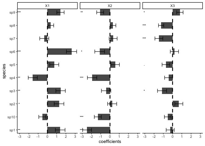
plot(model)
## Family:  binomial
##
## LogLik:  -510.9816
## Regularization loss:  0
##
## Species-species correlation matrix:
##
##  sp1  1.0000
##  sp2 -0.3780  1.0000
##  sp3 -0.2050 -0.4070  1.0000
##  sp4 -0.1850 -0.3860  0.8220  1.0000
##  sp5  0.6820 -0.4090 -0.1240 -0.0730  1.0000
##  sp6 -0.3050  0.4870  0.1630  0.1510 -0.1220  1.0000
##  sp7  0.5830 -0.1190  0.0960  0.1200  0.5520  0.2450  1.0000
##  sp8  0.3140  0.1690 -0.5280 -0.5460  0.2330 -0.0480  0.1300  1.0000
##  sp9 -0.0620 -0.0250  0.0840  0.0640 -0.4010 -0.3430 -0.2060 -0.1380  1.0000
##  sp10     0.2080  0.4750 -0.7140 -0.6490  0.2540  0.1410  0.1480  0.4560 -0.2850  1.0000
##
##
##
## Spatial:
##            sp1       sp2      sp3       sp4      sp5      sp6      sp7      sp8
## X1:X2 2.103188 -4.041381 3.452883 0.2332844 2.681165 1.325118 3.126471 1.928931
##             sp9     sp10
## X1:X2 0.9001696 1.262238
##
##
##
##                  Estimate Std.Err Z value Pr(>|z|)
## sp1 (Intercept)   -0.0847  0.2671   -0.32  0.75124
## sp1 X1             1.3854  0.5241    2.64  0.00820 **
## sp1 X2            -2.4736  0.4839   -5.11  3.2e-07 ***
## sp1 X3            -0.2583  0.4362   -0.59  0.55385
## sp2 (Intercept)   -0.0145  0.2601   -0.06  0.95560
## sp2 X1             1.2578  0.5233    2.40  0.01625 *
## sp2 X2             0.2357  0.4909    0.48  0.63112
## sp2 X3             0.6825  0.4302    1.59  0.11266
## sp3 (Intercept)   -0.5653  0.2861   -1.98  0.04819 *
## sp3 X1             1.4285  0.5099    2.80  0.00509 **
## sp3 X2            -0.4155  0.5096   -0.82  0.41489
## sp3 X3            -1.1364  0.4898   -2.32  0.02034 *
## sp4 (Intercept)   -0.1156  0.2580   -0.45  0.65406
## sp4 X1            -1.5792  0.4921   -3.21  0.00133 **
## sp4 X2            -1.9313  0.5088   -3.80  0.00015 ***
## sp4 X3            -0.4306  0.4314   -1.00  0.31822
## sp5 (Intercept)   -0.2109  0.2526   -0.83  0.40378
## sp5 X1             0.7425  0.4843    1.53  0.12525
## sp5 X2             0.5624  0.4582    1.23  0.21969
## sp5 X3            -0.7171  0.4154   -1.73  0.08433 .
## sp6 (Intercept)    0.2184  0.2707    0.81  0.41973
## sp6 X1             2.6087  0.5552    4.70  2.6e-06 ***
## sp6 X2            -1.1176  0.5271   -2.12  0.03400 *
## sp6 X3             0.2021  0.4461    0.45  0.65049
## sp7 (Intercept)   -0.0719  0.2448   -0.29  0.76903
## sp7 X1            -0.3372  0.4899   -0.69  0.49132
## sp7 X2             0.3403  0.4328    0.79  0.43175
## sp7 X3            -1.4822  0.4269   -3.47  0.00052 ***
## sp8 (Intercept)    0.1574  0.1625    0.97  0.33270
## sp8 X1             0.3657  0.3158    1.16  0.24688
## sp8 X2             0.3236  0.3102    1.04  0.29688
## sp8 X3            -1.2363  0.2850   -4.34  1.4e-05 ***
## sp9 (Intercept)    0.0235  0.2003    0.12  0.90667
## sp9 X1             1.4160  0.3943    3.59  0.00033 ***
## sp9 X2            -1.0606  0.3755   -2.82  0.00473 **
## sp9 X3             0.7943  0.3444    2.31  0.02111 *
## sp10 (Intercept)  -0.0825  0.2076   -0.40  0.69104
## sp10 X1           -0.5510  0.3781   -1.46  0.14505
## sp10 X2           -1.3145  0.3777   -3.48  0.00050 ***
## sp10 X3           -0.5257  0.3590   -1.46  0.14310
## ---
## Signif. codes:  0 '***' 0.001 '**' 0.01 '*' 0.05 '.' 0.1 ' ' 1
We support other distributions:
- Count data with Poisson:
model <- sjSDM(Y = Occ, env = linear(data = Env, formula = ~X1+X2+X3), spatial = linear(data = SP, formula = ~0+X1:X2), se = TRUE, family=poisson("log"))
- Count data with negative Binomial (which is still experimental, if you run into errors/problems, please let us know):
model <- sjSDM(Y = Occ, env = linear(data = Env, formula = ~X1+X2+X3), spatial = linear(data = SP, formula = ~0+X1:X2), se = TR, family="nbinom")
- Gaussian (normal):
model <- sjSDM(Y = Occ, env = linear(data = Env, formula = ~X1+X2+X3), spatial = linear(data = SP, formula = ~0+X1:X2), se = TR, family=gaussian("identity"))
Anova
ANOVA can be used to partition the three components (abiotic, biotic, and spatial):
an = anova(model)
print(an)
## Analysis of Deviance Table
##
## Terms added sequentially:
##
##           Deviance Residual deviance R2 Nagelkerke R2 McFadden
## Abiotic  157.95722        1177.48500       0.79394      0.1139
## Biotic   175.41278        1160.02944       0.82694      0.1265
## Spatial   17.38643        1318.05579       0.15959      0.0125
## Full     385.98836         949.45386       0.97893      0.2784
plot(an)
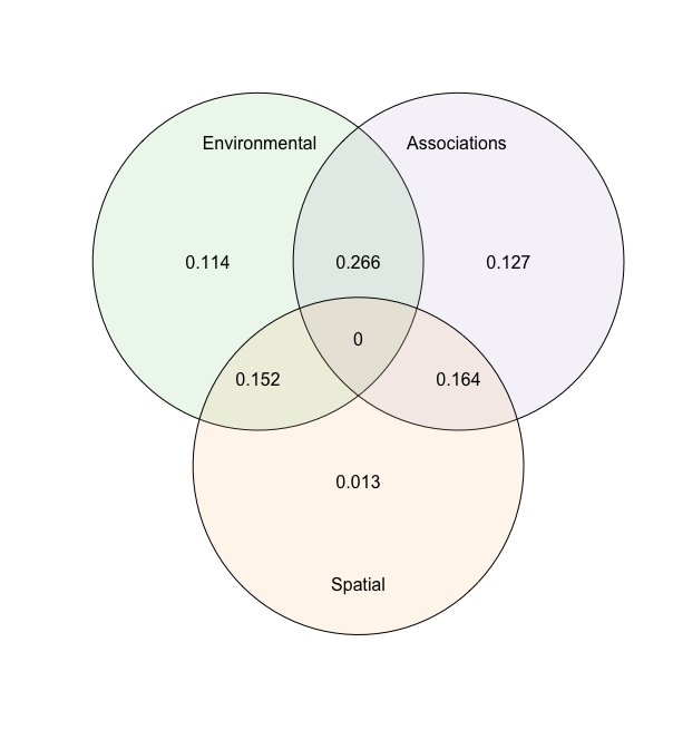
The anova shows the relative changes in the R2 of the groups and their intersections.
Internal metacommunity structure
Following Leibold et al., 2022 we can calculate and visualize the internal metacommunity structure (=partitioning of the three components for species and sites). The internal structure is already calculated by the ANOVA and we can visualize it with the plot method:
results = plotInternalStructure(an) # or plot(an, internal = TRUE)
## Registered S3 methods overwritten by 'ggtern':
##   method           from
##   grid.draw.ggplot ggplot2
##   plot.ggplot      ggplot2
##   print.ggplot     ggplot2
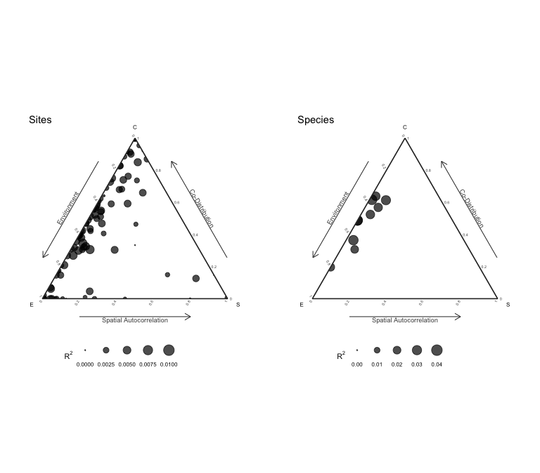
The plot function returns the results for the internal metacommunity structure:
print(results$data$Species)
##           env         spa     codist         r2
## 1  0.17677667 0.000000000 0.16810146 0.03375475
## 2  0.08724636 0.026656011 0.18072040 0.02946228
## 3  0.12613742 0.004529856 0.21004115 0.03407084
## 4  0.16648179 0.000000000 0.15890110 0.03241345
## 5  0.08585343 0.005811074 0.16168802 0.02533525
## 6  0.18787936 0.012341719 0.11489709 0.03151182
## 7  0.10765006 0.012898782 0.13292549 0.02534743
## 8  0.12445149 0.015040332 0.06188116 0.02013730
## 9  0.17762242 0.000000000 0.04357315 0.02196159
## 10 0.08805858 0.017406001 0.13890574 0.02443703
Installation trouble shooting
If the installation fails, check out the help of ?install_sjSDM, ?installation_help, and vignette(“Dependencies”, package = “sjSDM”).
- Try install_sjSDM()
- New session, if no ‘PyTorch not found’ appears it should work, otherwise see ?installation_help
- If do not get the pkg to run, create an issue issue tracker or write an email to maximilian.pichler at ur.de
Python Package
pip install sjSDM_py
Python example
import sjSDM_py as fa
import numpy as np
import torch
Env = np.random.randn(100, 5)
Occ = np.random.binomial(1, 0.5, [100, 10])

model = fa.Model_sjSDM(device=torch.device("cpu"), dtype=torch.float32)
model.add_env(5, 10)
model.build(5, optimizer=fa.optimizer_adamax(0.001),scheduler=False)
model.fit(Env, Occ, batch_size = 20, epochs = 10)
# print(model.weights)
# print(model.covariance)
## Iter: 0/10 0%| | [00:00, ?it/s]Iter: 0/10 0%| | [00:00, ?it/s, loss=7.17]Iter: 1/10 10%|# | [00:00, 3.88it/s, loss=7.17]Iter: 1/10 10%|# | [00:00, 3.88it/s, loss=7.158]Iter: 1/10 10%|# | [00:00, 3.88it/s, loss=7.149]Iter: 1/10 10%|# | [00:00, 3.88it/s, loss=7.142]Iter: 1/10 10%|# | [00:00, 3.88it/s, loss=7.124]Iter: 1/10 10%|# | [00:00, 3.88it/s, loss=7.118]Iter: 1/10 10%|# | [00:00, 3.88it/s, loss=7.112]Iter: 1/10 10%|# | [00:00, 3.88it/s, loss=7.108]Iter: 1/10 10%|# | [00:00, 3.88it/s, loss=7.118]Iter: 9/10 90%|######### | [00:00, 30.63it/s, loss=7.118]Iter: 9/10 90%|######### | [00:00, 30.63it/s, loss=7.144]Iter: 10/10 100%|##########| [00:00, 26.74it/s, loss=7.144]
Calculate Importance:
Beta = np.transpose(model.env_weights[0])
Sigma = ( model.sigma @ model.sigma.t() + torch.diag(torch.ones([1])) ).data.cpu().numpy()
covX = fa.covariance( torch.tensor(Env).t() ).data.cpu().numpy()

fa.importance(beta=Beta, covX=covX, sigma=Sigma)
## {'env': array([[ 1.2717709e-02,  7.8437300e-03,  6.6514793e-03, -3.3015787e-04,
##          2.3806898e-04],
##        [ 9.9158729e-05, -1.8891758e-06,  1.0537009e-03,  4.0511694e-04,
##          1.1120385e-02],
##        [ 6.1564189e-03,  5.9850062e-03,  9.2307013e-03,  5.4843356e-03,
##         -3.3683516e-04],
##        [ 1.3349474e-02,  4.3294221e-04,  1.8103119e-03,  1.4068705e-02,
##          6.6316797e-04],
##        [ 3.3953122e-05,  3.1304134e-03,  2.6658648e-03, -3.6165391e-05,
##          7.3677581e-03],
##        [ 2.7722977e-03,  1.9519718e-03,  4.8086399e-04,  3.0876237e-03,
##          1.7828522e-04],
##        [ 7.9284189e-03,  5.7881157e-04,  7.5722663e-03,  2.1802005e-06,
##          4.2433664e-03],
##        [-5.1329907e-06,  6.0144444e-03,  2.1059261e-05,  7.5954124e-03,
##          1.5537007e-03],
##        [ 7.7161851e-04,  1.7209088e-02,  4.8407568e-03,  1.8020724e-03,
##          5.6920521e-04],
##        [ 1.7108561e-02,  7.2742125e-04,  9.4651995e-04,  6.8342132e-03,
##          1.1830850e-02]], dtype=float32), 'biotic': array([0.9728792 , 0.9873236 , 0.9734804 , 0.9696754 , 0.9868381 ,
##        0.9915289 , 0.97967494, 0.9848205 , 0.9748072 , 0.9625524 ],
##       dtype=float32)}