[4]{.chapter-number}  [Linear mixed models]{.chapter-title}

4 Linear mixed models

4.1 Motivation

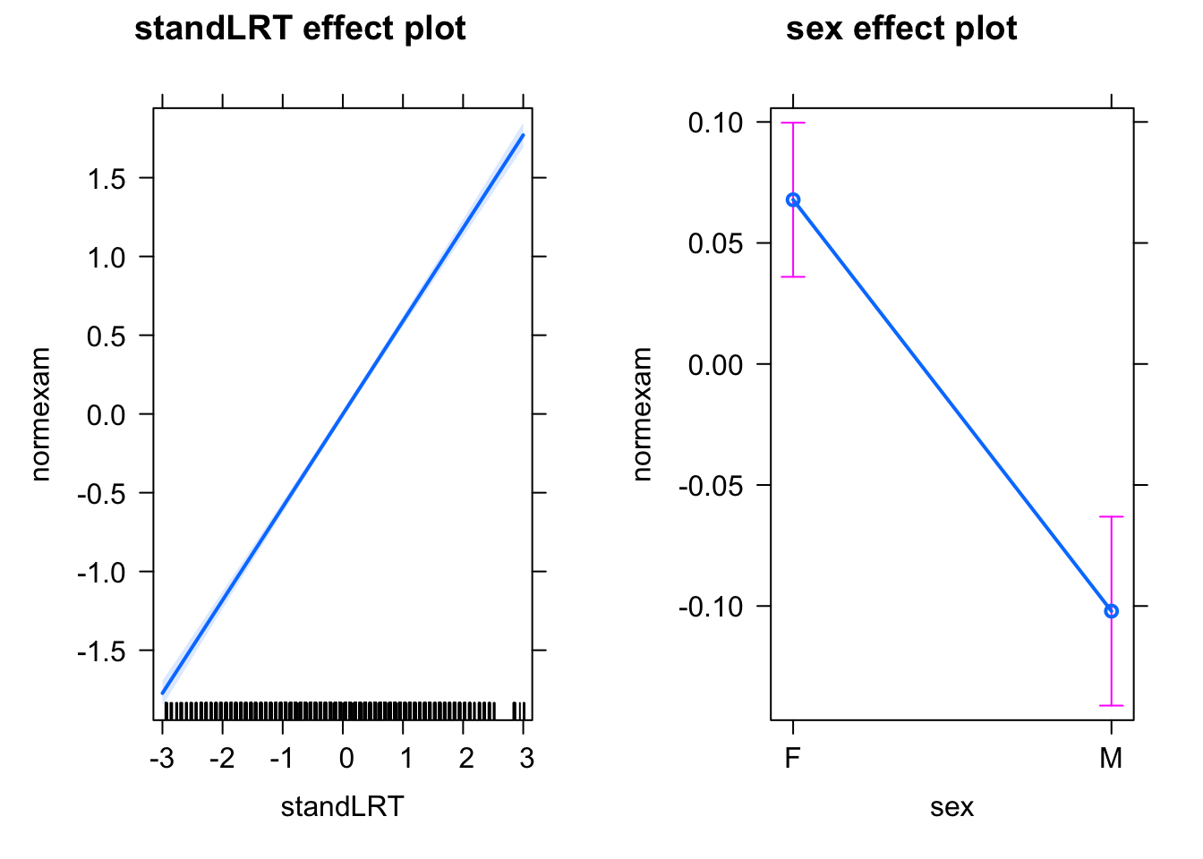
Random effects are a very common addition to regression models that are used to account for grouping (categorical) variables such as subject, year, location. To explain the motivation for these models, as well as the basic syntax, we will use an example data set containing exam scores of 4,059 students from 65 schools in Inner London. This data set is located in the R package mlmRev.

Response: “normexam” (Normalized exam score).
Predictor 1: “standLRT” (Standardised LR test score; Reading test taken when they were 11 years old).
Predictor 2: “sex” of the student (F / M).
Grouping factor: school

If we analyze this with a simple LM, we see that reading ability and sex have the expected effects on the exam score.

library(mlmRev)
library(effects)

mod0 = lm(normexam ~ standLRT + sex , data = Exam)
plot(allEffects(mod0))

However, it is reasonable to assume that not all schools are equally good, which has two possible consequences:

If school identity correlates with sex or standLRT, school could be a confounder (more on this later)
Residuals will be correlated in school, thus they are not iid (pseudo-replication)

We could solve this problem by fitting a different mean per school

mod0b = lm(normexam ~ standLRT + sex + school , data = Exam)

however, with 65 schools this would cost 64 degrees of freedom, which is a high cost just for correcting the possibility of confounding and a minor residual problem.

The solution: Mixed / random effect models. In a mixed model, we assume (differently to a fixed effect model) that the variance between schools originates from a normal distribution. There are different interpretations of a random effect (more on this later), but one interpretation is to view the random effect as an additional error, so that such a mixed model has two levels of error:

First, the random effect, which is a normal “error” acting on an entire group of data points (in this case school).
And second, the residual error, which is a normal error per observation and acts on top of the random effect

Because of this hierarchical structure, these models are also called “multi-level models” or “hierarchical models”.

Note

Because grouping naturally occurs in any type of experimental data (batches, blocks, observer, subject etc.), random and mixed effect models are the de-facto default for most experimental data! Naming conventions:

No random effect = fixed effect model
Only random effects = random effect model
Random effects + fixed effects = mixed model

Most models that are used in practice are mixed models

4.2 Specifying and estimating mixed models:

4.2.1 The random intercept model

The simplest random effect structure is the random intercept model.

Each random effect model has a fixed counterpart. For the random intercept model, this counterpart is the model we already saw, with school as a fixed effect

mod0b = lm(normexam ~ standLRT + sex + school , data = Exam)

The random intercept model is practically identical to the model above, except that it assumes that the school effects come from a common normal distribution. The model can be estimated with lme4::lmer

library(lme4)
mod1 = lmer(normexam ~ standLRT + sex +  (1 | school/student), data = Exam)

boundary (singular) fit: see help('isSingular')

summary(mod1)

Linear mixed model fit by REML ['lmerMod']
Formula: normexam ~ standLRT + sex + (1 | school/student)
   Data: Exam

REML criterion at convergence: 9346.6

Scaled residuals: 
    Min      1Q  Median      3Q     Max 
-3.7120 -0.6314  0.0166  0.6855  3.2735 

Random effects:
 Groups         Name        Variance Std.Dev.
 student:school (Intercept) 0.00000  0.0000  
 school         (Intercept) 0.08986  0.2998  
 Residual                   0.56252  0.7500  
Number of obs: 4059, groups:  student:school, 4055; school, 65

Fixed effects:
            Estimate Std. Error t value
(Intercept)  0.07639    0.04202   1.818
standLRT     0.55947    0.01245  44.930
sexM        -0.17136    0.03279  -5.226

Correlation of Fixed Effects:
         (Intr) stnLRT
standLRT -0.013       
sexM     -0.337  0.061
optimizer (nloptwrap) convergence code: 0 (OK)
boundary (singular) fit: see help('isSingular')

If we look at the outputs, you will probably note that the summary() function doesn’t return p-values. More on this in the section on problems and solutions for mixed models. Also, we see that the effects of the individual school are not explicitly mentioned. The summary only returns the mean effects over all schools, and the variance between schools. However, you can obtain the individual school effects via

ranef(mod1)

Moreover, unlike the outputs we have seen before, the model also returns a correlation between fixed effect estimates. This, however, is simply a choice of the programmers, it has nothing to do with the random effect models - you could calculate the same output for the lm() via the function vcov().

Here is a visualization of the fitted effects for standLRT

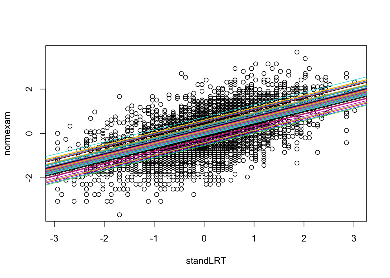
We can see that there is the same slope, but a different intercept per school.

The RE effectively “centers” the categorical predictor - unlike for the fixed effect model, where the intercept would be interpreted as the value for the first school, the intercept in the random effect model is the mean across all schools, and the REs measure the deviation of the individual school from the mean. It should be stressed, however, that this is a welcome consequence, but not the main motivation, for the RE structure.

Generate equation with the equatiomatic package

We can use the equatiomatic package to print LaTeX code for the underlying equation of our random intercept model:

library(equatiomatic)
extract_eq(mod1)

\[ \begin{aligned} \operatorname{normexam}_{i} &\sim N \left(\alpha_{j[i]} + \beta_{1}(\operatorname{standLRT}) + \beta_{2}(\operatorname{sex}_{\operatorname{M}}), \sigma^2 \right) \\ \alpha_{j} &\sim N \left(\mu_{\alpha_{j}}, \sigma^2_{\alpha_{j}} \right) \text{, for school j = 1,} \dots \text{,J} \end{aligned} \]

4.2.2 The random slope model

A second effect that we could imagine is that the effect of standLRT is different for each school. As a fixed effect model, we would express this, for example, as lm(normexam ~ standLRT*school + sex)

The random effect equivalent is called the random slope model. A random slope model assumes that each school also gets their own slope for a given parameter (per default we will always estimate slope and intercept, but you could overwrite this, not recommended!). Let’s do this for standLRT (you could of course random slopes on both predictors as well).

mod2 = lmer(normexam ~ standLRT + sex +  (standLRT | school), data = Exam)
summary(mod2)

Linear mixed model fit by REML ['lmerMod']
Formula: normexam ~ standLRT + sex + (standLRT | school)
   Data: Exam

REML criterion at convergence: 9303.2

Scaled residuals: 
    Min      1Q  Median      3Q     Max 
-3.8339 -0.6373  0.0245  0.6819  3.4500 

Random effects:
 Groups   Name        Variance Std.Dev. Corr
 school   (Intercept) 0.08795  0.2966       
          standLRT    0.01514  0.1230   0.53
 Residual             0.55019  0.7417       
Number of obs: 4059, groups:  school, 65

Fixed effects:
            Estimate Std. Error t value
(Intercept)  0.06389    0.04167   1.533
standLRT     0.55275    0.02016  27.420
sexM        -0.17576    0.03228  -5.445

Correlation of Fixed Effects:
         (Intr) stnLRT
standLRT  0.356       
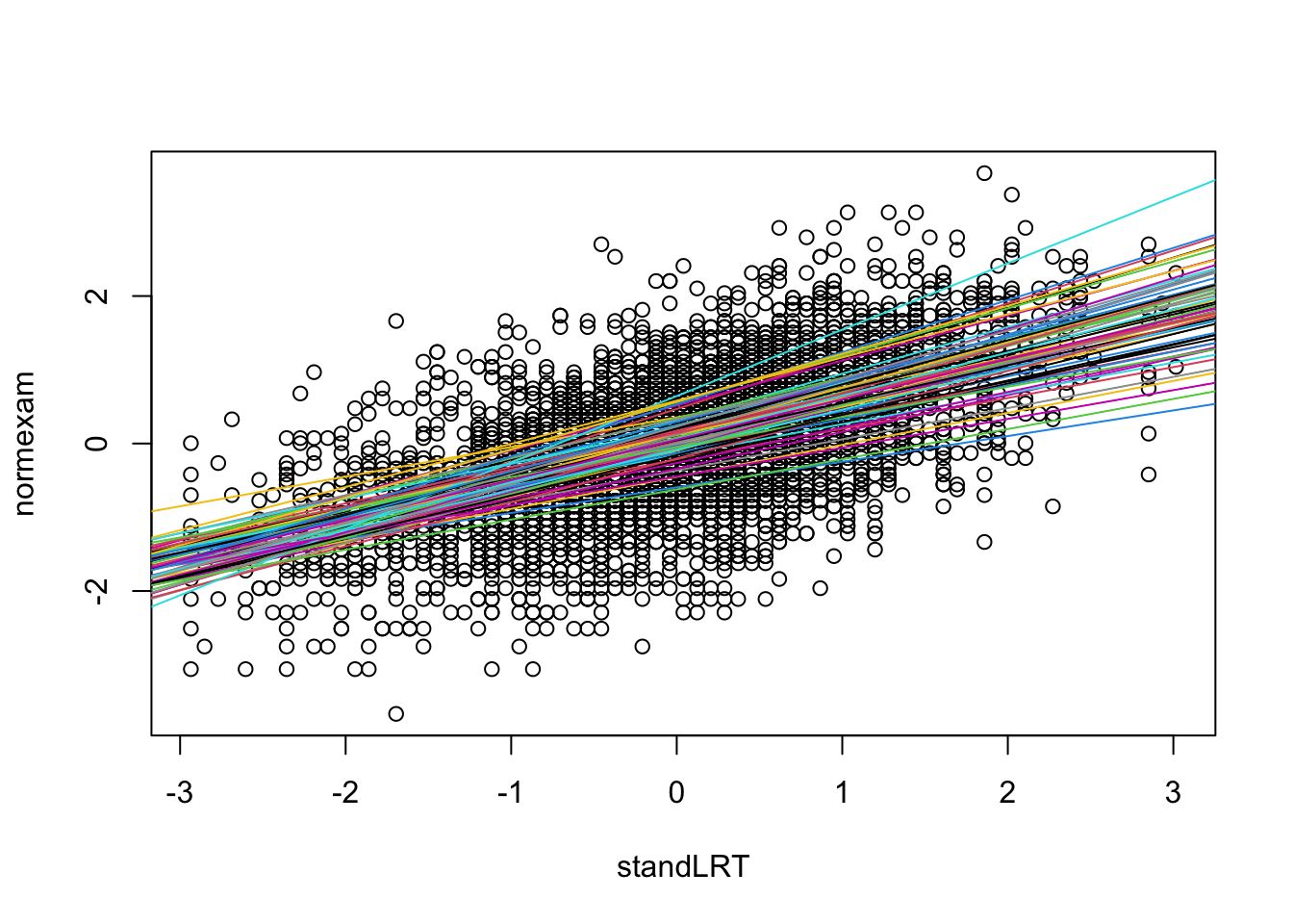
sexM     -0.334  0.036

Again, the difference to the fixed effect model is that in the random effect model, we assume that the variance between slopes come from a normal distribution. The results is similar to the random intercept model, except that we have an additional variance term for the slopes, and a term for the interaction between slopes and intercepts.

Generate equation with the equatiomatic package

We can use the equatiomatic package to print LaTeX code for the underlying equation of our random slope model:

library(equatiomatic)
extract_eq(mod2)

\[ \begin{aligned} \operatorname{normexam}_{i} &\sim N \left(\alpha_{j[i]} + \beta_{1j[i]}(\operatorname{standLRT}) + \beta_{2}(\operatorname{sex}_{\operatorname{M}}), \sigma^2 \right) \\ \left( \begin{array}{c} \begin{aligned} &\alpha_{j} \\ &\beta_{1j} \end{aligned} \end{array} \right) &\sim N \left( \left( \begin{array}{c} \begin{aligned} &\mu_{\alpha_{j}} \\ &\mu_{\beta_{1j}} \end{aligned} \end{array} \right) , \left( \begin{array}{cc} \sigma^2_{\alpha_{j}} & \rho_{\alpha_{j}\beta_{1j}} \\ \rho_{\beta_{1j}\alpha_{j}} & \sigma^2_{\beta_{1j}} \end{array} \right) \right) \text{, for school j = 1,} \dots \text{,J} \end{aligned} \]

Here a visualization of the results

with(Exam, {
  randcoefI = ranef(mod2)$school[,1]
  randcoefS = ranef(mod2)$school[,2]
  fixedcoef = fixef(mod2)
  plot(standLRT, normexam)
    for(i in 1:65){
      abline(a = fixedcoef[1] + randcoefI[i] , b = fixedcoef[2] + randcoefS[i], col = i)
    }
})

4.2.3 Mixed models in different packages

4.2.3.1 lme4 / glmmTMB

There are a large number of packages to fit mixed models in R. The main packages that you use, because they are most user-friendly and stable, are lme4 and glmmTMB. They share more or less the same syntax for random effects.

Random intercept: (1 | group).
ONLY random slope for a given fixed effect: (0 + fixedEffect | group).
Random slope + intercept + correlation (default): (fixedEffect | group).
Random slope + intercept without correlation: (fixedEffect || group), identical to
(1 | group) + (0 + fixedEffect | group).
Nested random effects: (1 | group / subgroup). If groups are labeled A, B, C, … and subgroups 1, 2, 3, …, this will create labels A1, A2 ,B1, B2, so that you effectively group in subgroups. Useful for the many experimental people that do not label subgroups uniquely, but otherwise no statistical difference to a normal (crossed) random effect.
Crossed random effects: You can add random effects independently, as in
(1 | group1) + (1 | group2).

4.2.3.2 nlme

nlme is a classic package for fitting (nonlinear) mixed effect models. I would argue that it is largely superseded by lme4 and glmmTMB, but it still offers a few special tricks that are not available in either lme4 or glmmTMB. A linear mixed model with random intercept in nlme looks like this

nlme::lme(Resp ~ Predictor, random=~1|Group)

4.2.3.3 mgcv

If you want to use GAMs, there is basically only mgcv (or brms, if you’re willing to go Bayesian).

mgcv::gam(Resp ~ Predictor + s(Group, bs = 're'))

4.2.3.4 brms

brms is a very interesting package that allows to estimate mixed models via Bayesian Inference with STAN.

brms::brm(Resp ~ Predictor + (1|Group),
         data = Owls , family = poisson)
summary(mod1)

4.2.4 REML vs. MLE

Frequentist linear mixed models are usually estimated with REML = restricted maximum likelihood, rather than with classical MLE. Most packages allow you to switch between REML and MLE. The motivation for REML is that for limited data (non-asymptotics), the MLE for variance components of the model are typically negatively biased, because the uncertainty of the fixed effects is not properly accounted for. If you go through the mathematics, you can make an analogy to the bias-corrected sampling variance (Bates 2011).

REML uses a mathematical transformation to first obtain the residuals conditional on the fixed effect components of the model (thus accounting for the df lost in this part), and then estimating variance components. One can view REML as a special case of an expectation maximization (EM) algorithm.

Most packages offer an option to switch between REML and ML estimation of the model. In lme4, this is done via

Regarding when to use what, use the following rule of thumb:

Per default, use REML
Switch to ML if you use downstream any model functions that use the likelihood, unless you are really sure that the calculation you do is also valid for REML.

Tip

In later in this chapter, we will talk about model selection via LRTs and AIC. Because those depend on the likelihood, it is generally recommended to switch from REML to ML in this case. The reason is that, because REML estimates the REs conditional on the fixed effects, REML likelihoods are not directly comparable if fixed effects are changed. I would recommend to stick to this, although I have to say that I have always wondered how big this problem is, compared to the other df problems associated to mixed models (see below).

4.2.5 Exercise

Excercise: a mixed model for plantHeight

Take plantHeight model that we worked with already:

library(EcoData)

oldModel <- lm(loght ~ temp, data = plantHeight)
summary(oldModel)

We have one observation per species. Consider that the relationship height ~ temp may be different for each family. Some families may have larger plants in general (random intercept), but it may also be that the temperature relationship changes per family (random slope). Run these two models for our problem.

Solution

# Random intercept model

library(lme4)
library(lmerTest)
randomInterceptModel <- lmer(loght ~ temp + (1|Family), data = plantHeight)
summary(randomInterceptModel)

# Random slope model

randomSlopeModel <- lmer(loght ~ temp + (temp | Family), data = plantHeight)
summary(randomSlopeModel)

# scaling helps the optimizer
plantHeight$sTemp = scale(plantHeight$temp)

randomSlopeModel <- lmer(loght ~ sTemp + (sTemp | Family), data = plantHeight)
summary(randomSlopeModel)

4.3 Advantages and interpretation of random effects

What do the random effects mean, and why should we use them?

4.3.1 Interpretation

The classical interpretation of the random intercept is that they model a group-structured residual error, i.e. they are like residuals, but for an entire group. However, this view breaks down a bit for a random slope model.

Another view this is that REs terms absorb group-structured variation in model parameters. This view works for random intercept and slope models. So, our main model fits the grand mean, and the RE models variation in the parameters, which is assumed to be normally distributed.

A third view of RE models is that they are regularized fixed effect models. What does that mean? Note again that, conceptual, every random effect model corresponds to a fixed effect model. For a random intercept model, this would be

lmer(y ~ x + (1|group)) => lm(y ~ x + group)

and for the random slope, it would be

lmer(y ~ x + (x|group)) => lm(y ~ x * group)

So, alternatively to a mixed model, we could always fit a fixed effect model, and that would also take care of the variation in groups. Of course, the output of the two models differs, but that’s just what people programmed. The real difference, however, is that by making the assumption that the random effects come from a normal distribution, we are imposing a constraint on the estimates, which creates a shrinkage on the fitted REs (see below).

4.3.2 RE shrinkage

To understand shrinkage, note that whatever the fitted sd of the normal distribution underlying the RE, as long as it is finite, it will always be more likely that the RE estimate is at zero (i.e. the grand mean) than at 1 or 2 sd. This means that RE estimates are biased towards the grand mean.

We can visualize the effect by comparing estimates of a fixed to a random effect model

mf = lm(normexam ~ 0 + school, data = Exam)
mr = lmer(normexam ~ (1 | school), data = Exam)

ef = coef(mf)
er = ranef(mr)$school$`(Intercept)`
plot(ef, er, xlab = "fixed", ylab = "random")
abline(0,1)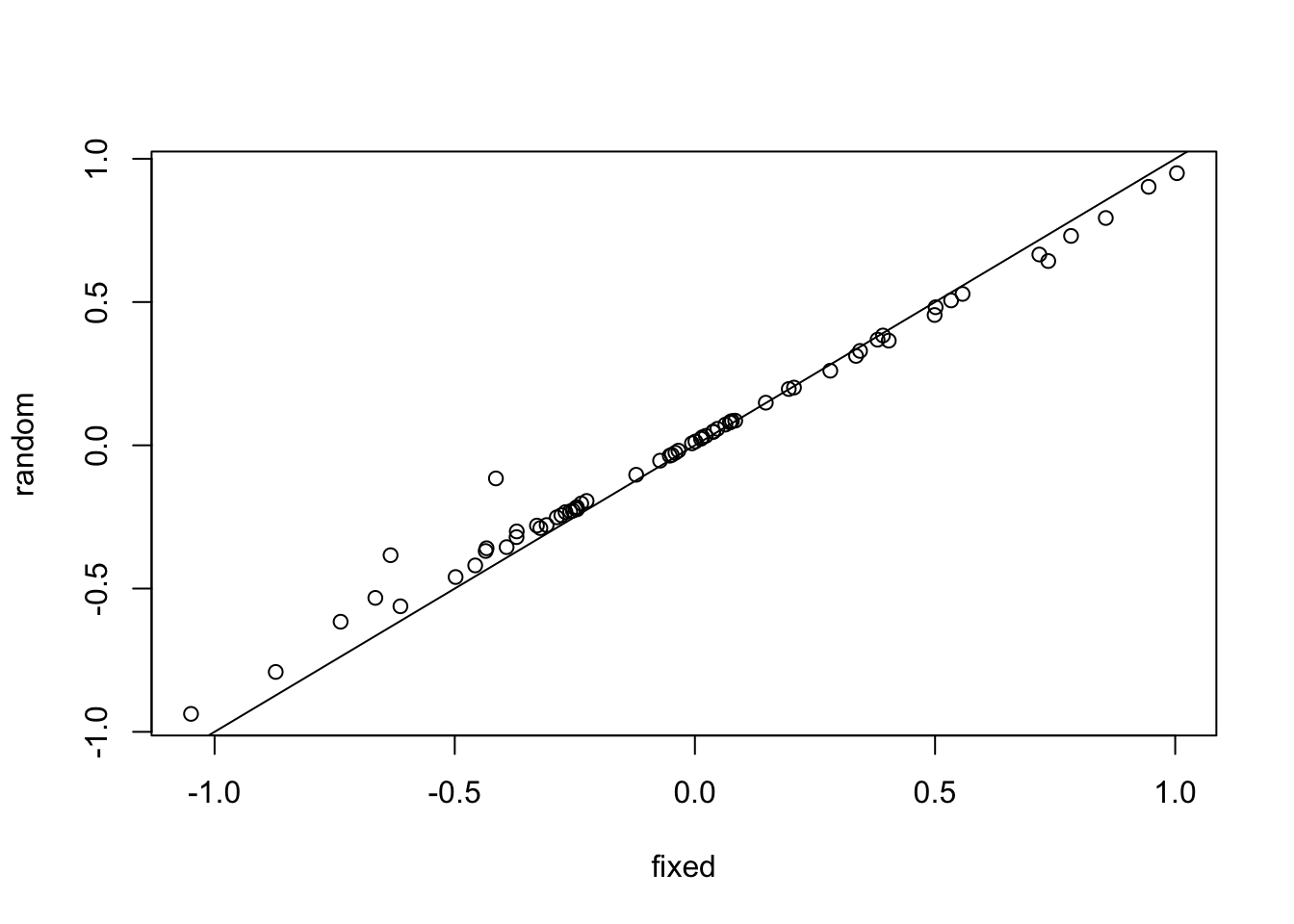

The plot shows that random effect estimates are biased towards the grand mean, i.e. positive values are lower than in the LM, and negative values are higher than in the LM. This is called shrinkage.

Note

The shrinkage imposed by the RE is equivalent to an L2 (ridge) regression (see section on model selection), or a normally distributed Bayesian prior. You can see this by considering that the log likelihood of a normal distribution is equivalent to a quadratic penalty for deviations from the mean. The difference is that the strength of the penalty, controlled by the RE sd, is estimated. For that reason, the RE shrinkage is also referred to as an example of “adaptive shrinkage”.

This RE shrinkage is useful in many situations, beyond describing a group-structured error in the data. A common use is that by using a random slope model, parameter estimates for groups with few data points are drawn towards the grand mean and thus informed by the estimates of the other groups. For example, if we have data for common and rare species, and we are interested in the density dependence of the species, we could fit. Consider the plantHeight case study we did in the section on linear regression. We saw that, even after re-leveling the predictor, not all interactions could be estimated, because some factor levels had only one observation.

library(EcoData)
plantHeight$growthform2 = relevel(as.factor(plantHeight$growthform), "Herb")
plantHeight$sTemp = scale(plantHeight$temp)
fit <- lm(loght ~ sTemp * growthform2 , data = plantHeight)
summary(fit)

If you run the same thing as a random slope model, you will see that we can estimate a random intercept and slope for each species, even those that have only one observation

fit <- lmer(loght ~ sTemp + (sTemp | growthform2) , data = plantHeight)
ranef(fit)

$growthform2
           (Intercept)       sTemp
Herb       -0.70060787  0.07032554
Fern       -0.07771756  0.01484118
Herb/Shrub -0.18519919  0.03351554
Shrub      -0.17681675  0.11176808
Shrub/Tree  0.29044226 -0.04361958
Tree        0.84989911 -0.18683076

with conditional variances for "growthform2"

The reason is that rare growth forms will be constrained by the RE, while common growth forms with a lot of data can overrule the normal distribution imposed by the random slope and get their own estimate. In this picture, the random effect imposes an adaptive shrinkage, similar to a LASSO or ridge shrinkage estimator, with the shrinkage strength controlled by the standard deviation of the random effect. An alternative view is that the RE variance acts as a prior distribution on the slope. Of course, estimates are biased towards zero, so if you want to interpret these estimatest that is a cost that you have to take into account.

4.3.3 When to use what?

So, to finalize this discussion: there are essentially two main differences between a random vs. fixed effect model

In the RE model, we are fitting a grand mean and differences from the grand mean, while in the fixed effect model, we have to set up contrasts (various options), with treatment contrasts as defaults
The LM (OLS) is mathematically proven to be the best linear unbiased estimator (BLUE) of the regression problem. In a mixed model, REs (but not fixed effects) are biased towards the grand mean, but the advantage is that the random effect looses less degrees of freedom, i.e. the power on the fixed effects will be higher.

While point 1 is more a choice about how to report results (in principle, we could also calculate the grand mean for fixed effect group estimates), the second point (higher power) is a clear advantage in many cases, in particular if you don’t care about the bias on the REs. Therefore, the rule of thumb for REs is:

If you have a categorical variable, and you’re not interested in it’s estimates, model it as a RE
If you want to get unbiased estimates of the categorical variable (or its interactions), use a fixed effect

This is just a rule of thumb, as said, in data-poor situations, it is common to use random slope models and interpret the estimates as well. In this case, we are using the RE to optimize the bias-variance trade-off (see chapter on model selection).

4.4 Model checks

As residual checks for an LMM, you should first of all check for everything that you would check in an LM, i.e. you would expect that the residual distribution is iid normal. On top of that, you should check the REs for:

Convergence (mixed models often have convergence problems)
Normality
Correlation with predictors -> RE can mask misfit
Residual patterns -> evidence for random slope

I will show all of those using the example

mod1 = lmer(normexam ~ standLRT + sex +  (1 | school), data = Exam)
summary(mod1)

Linear mixed model fit by REML ['lmerMod']
Formula: normexam ~ standLRT + sex + (1 | school)
   Data: Exam

REML criterion at convergence: 9346.6

Scaled residuals: 
    Min      1Q  Median      3Q     Max 
-3.7120 -0.6314  0.0166  0.6855  3.2735 

Random effects:
 Groups   Name        Variance Std.Dev.
 school   (Intercept) 0.08986  0.2998  
 Residual             0.56252  0.7500  
Number of obs: 4059, groups:  school, 65

Fixed effects:
            Estimate Std. Error t value
(Intercept)  0.07639    0.04202   1.818
standLRT     0.55947    0.01245  44.930
sexM        -0.17136    0.03279  -5.226

Correlation of Fixed Effects:
         (Intr) stnLRT
standLRT -0.013       
sexM     -0.337  0.061

4.4.1 Convergence

If there is a convergence problem, you should usually get a warning. Other signs of convergence problems may be RE estimates that are zero, CIs that are extremely large, or strong correlations in the correlation matrix of the predictors that is reported by summary(). Here, we have no problems, but we’ll see examples of this as we go on.

There are different types of convergence problems that you can encounter:

Warnings about scaling and centering -> just do it, it doesn’t cost you!
The warning “boundary (singular) fit: see help(‘isSingular’)” (meaning that some dimensions of the variance-covariance matrix have been estimated to zero. -> often, this just means that a RE estimate is zero. In many cases, this is not a problem and can actually be ignored, but it is hard to give general advice to when this is the case. In random slope models, it often helps to move from | to || (supressing the correlation). Removing the RE will solve the problem, but could lead to type I error inflation. A more conservative solution would be to change the RE to a fixed effect
Optimizer / convergence warnings: use glmerControl() to change the optimizer to bobyqa and possibly increase the number of iterations.

4.4.2 Observation-level residual plots

Unfortunately, lme4 plots only provide res ~ fitted as default

plot(mod1)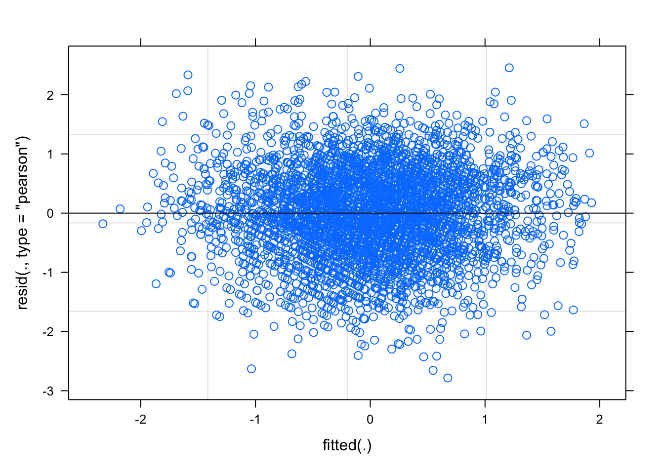

For a qqplot, you have to calculate the residuals by hand

qqnorm(residuals(mod1))
qqline(residuals(mod1))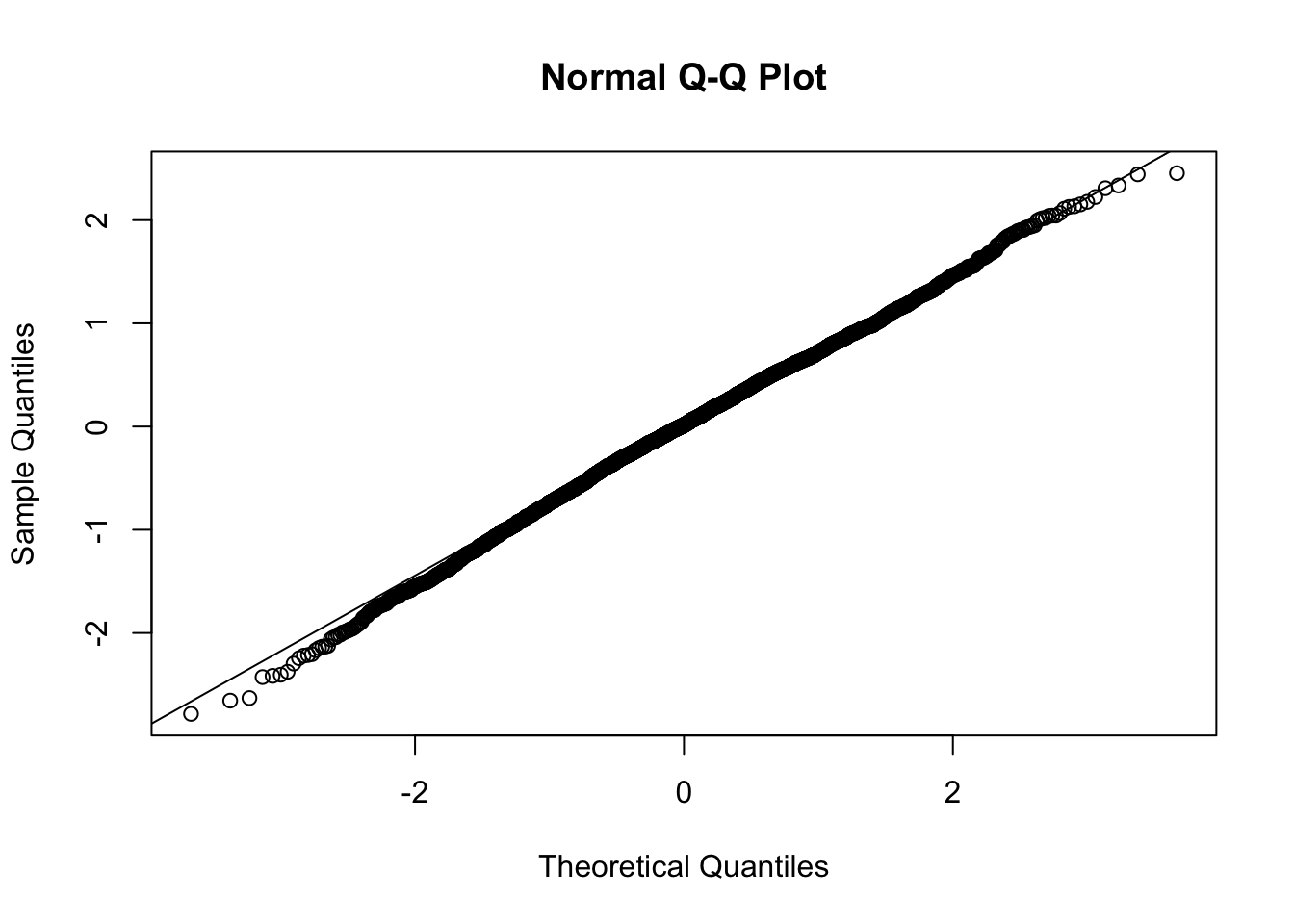

Of course, any time you do a qqnorm plot, you could also run a shapiro.test to get a p-value for the deviation from normality. You can also use the DHARMa plots

library(DHARMa)

This is DHARMa 0.4.7. For overview type '?DHARMa'. For recent changes, type news(package = 'DHARMa')

res <- simulateResiduals(mod1, plot = T)

Both plots look fine. Of course, we should also check residuals against predictors. In DHARMa, we can do this via

par(mfrow = c(1,2))
plotResiduals(res, Exam$standLRT)
plotResiduals(res, Exam$sex)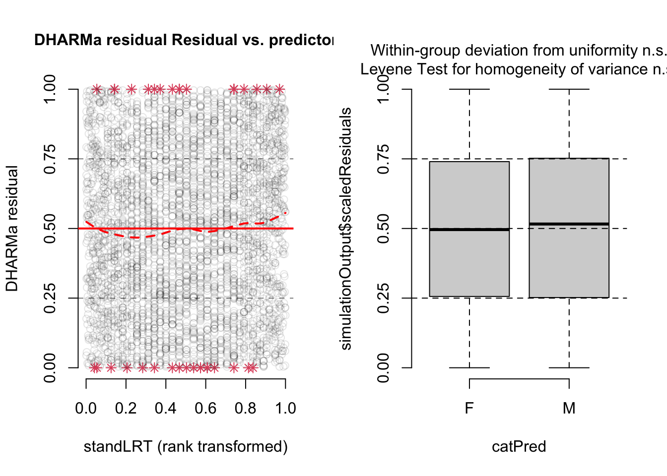

Tip

When you predict with a random effect model, you can do conditional or marginal predictions. The difference is that conditional predictions include the REs, while marginal predictions only include the fixed effects.

residuals(mod1, re.form = NULL) # conditional, default
predict(mod1, re.form = ~0) # marginal

This also makes a difference for the residual calculations: in principle, you could calculate residuals with respect to both predictions. In practice, the default in lme4 is to calculate residual predictions

residuals(mod1)
Exam$normexam - predict(mod1, re.form = NULL) 
Exam$normexam - predict(mod1, re.form = ~0)

while the default in DHARMa is to calculate marginal predictions. Both has advantages and disadvantages:

Conditional predictions are more sensitive to violations of the iid normal assumptions of the outer (observation-level) normal error
However, REs can sometimes absorb misfit, such that plotting conditional residuals ~ pred looks fine, but uncoditional ~ pred does not. For that reason, if you use unconditional predictions, you should also check REs ~ pred (see below)

4.4.3 Normality of REs

I prefer to look at this visually. You can also run a shapiro.test() to check if you should consider the pattern at all.

x = ranef(mod1)
qqnorm(x$school$`(Intercept)`)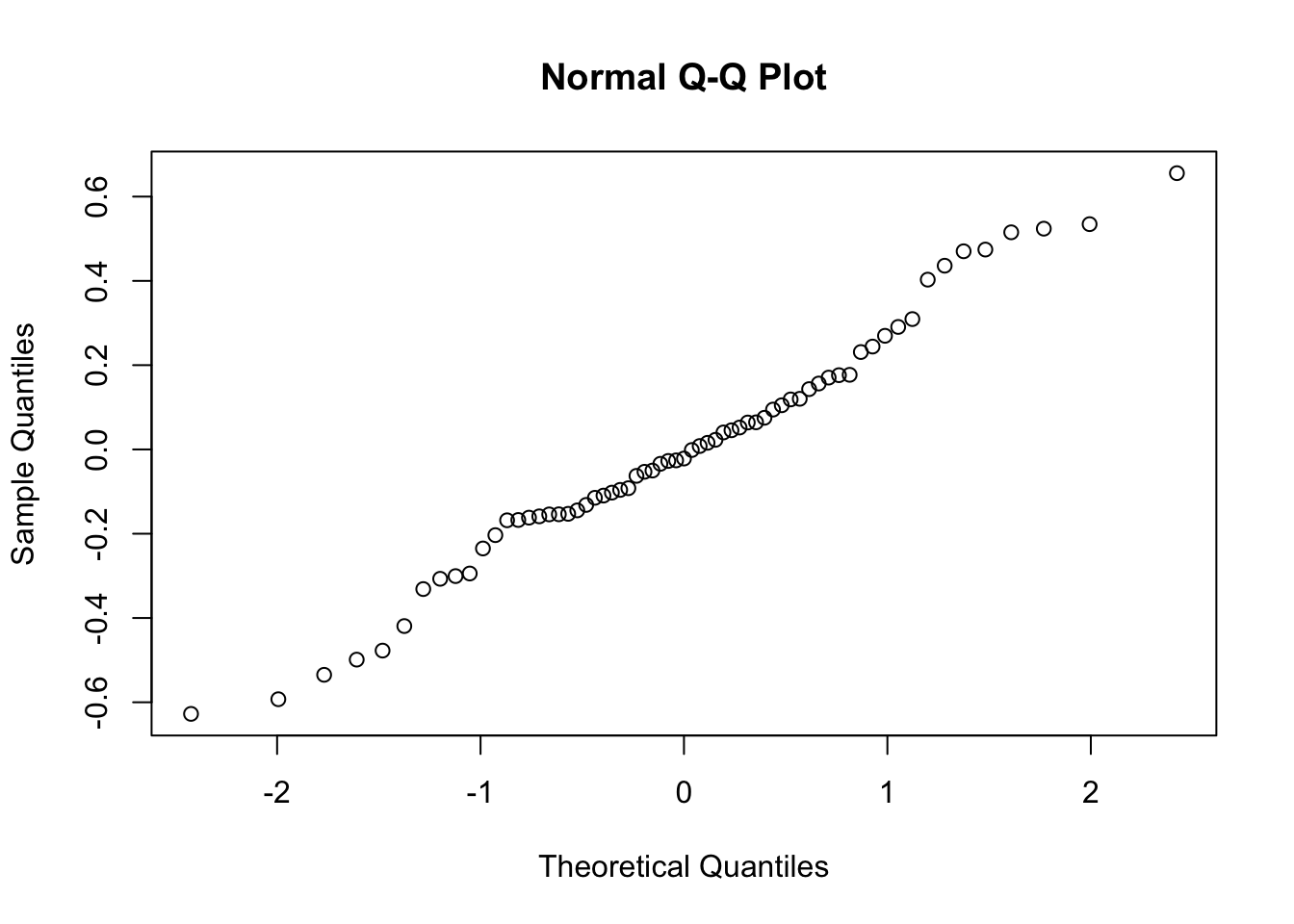

Question is how bad can this be? (Neuhaus, McCulloch, and Boylan 2013) report some simulation results that suggest that fixed effect slopes (bias, coverage) are relatively robust to misspecification in the RE distribution, which is re-assuring.

4.4.4 Correlation of REs with predictors

As mentioned above, REs can sometimes absorb misfit of the fixed effect structure. It can therefore be useful to check if there is a correlation with the predictors, especially if you only check conditional residuals. Example:

y = aggregate(cbind(standLRT, sex) ~ school, FUN = mean, data = Exam)
plot(x$school$`(Intercept)` ~ y$standLRT)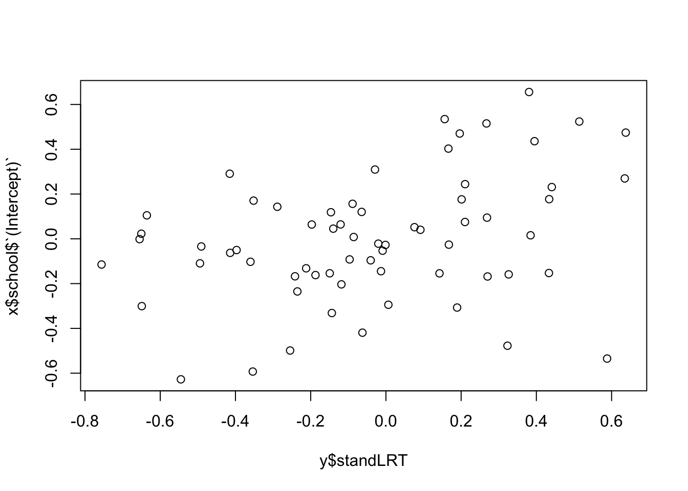

4.4.5 Residual pattern per group

lme4 has an excellent plot syntax to plot residuals per grouping factor. Check out the help of plot.merMod. The following plot shows residuals ~ fitted for each school

plot(mod1, resid(., scaled=TRUE) ~ standLRT | school, abline = 0)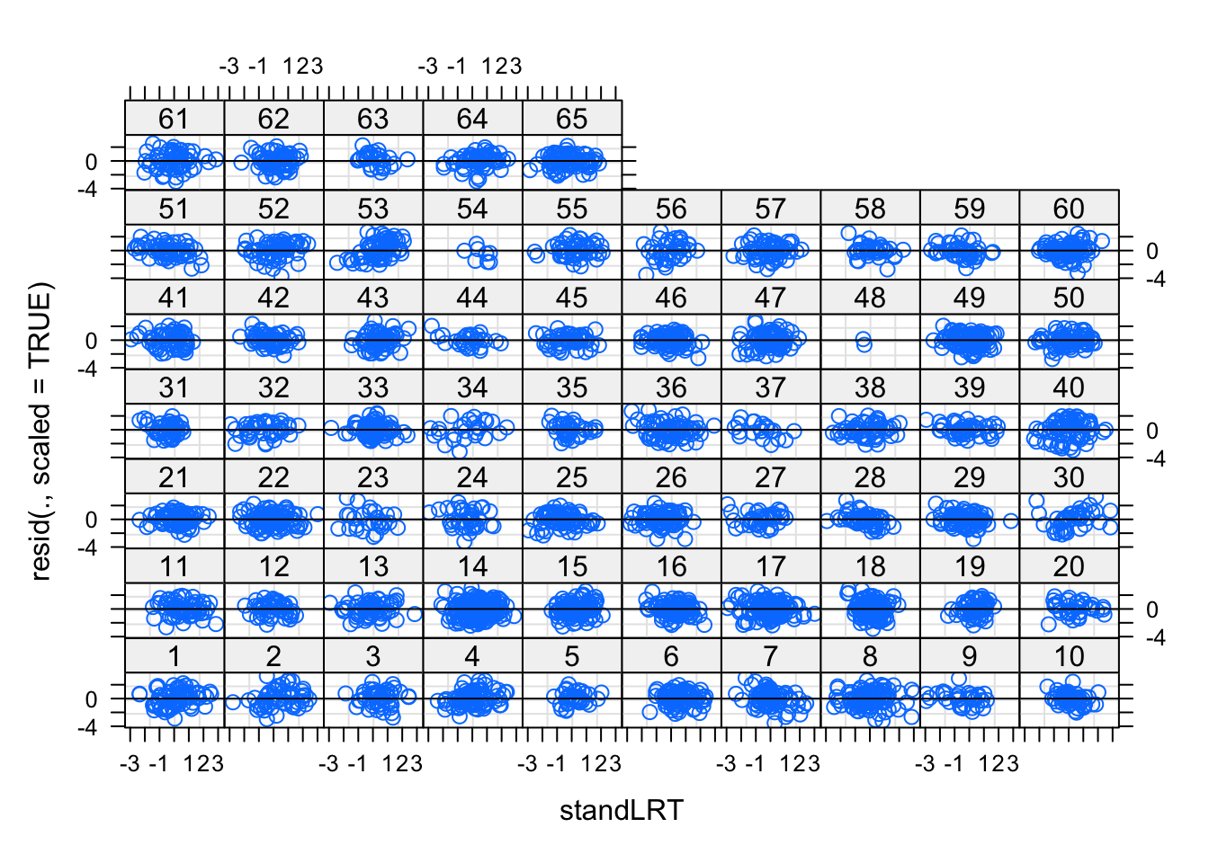

Looks still good to me, but if we think we see a pattern here, we should introduce a random slope.

4.5 Downstream Analysis of Mixed Models

Specifying mixed models is quite simple, however, there is a large list of (partly quite complicate) issues in their practical application. Here, a (incomplete) list:

4.5.1 Degrees of freedom for a random effect

Possibly the most central problem is: How many parameters does a random effect model have?

Note

Why is it so important to know how many parameters a model has? The answer is that what seems like a very minor point is needed in all the mathematics for calculating p-values, AIC, LRTs and all that, so without knowing the complexity of the model, the mathematics that is used in lm() breaks down.

We can make some guesses about the complexity of an LMM by looking at its fixed effect version counterparts:

mod1 = lm(normexam ~ standLRT + sex , data = Exam)
mod1$rank # 3 parameters.

mod2 = lmer(normexam ~ standLRT + sex +  (1 | school), data = Exam)
# No idea how many parameters.

mod3 = lm(normexam ~ standLRT + sex + school, data = Exam)
mod3$rank # 67 parameters.

So, we see that the fixed effect model without school has 3 parameters, and with school 67. It is reasonable to assume that the complexity of the mixed model is somewhere in-between, because it fits the same effects as mod3, but they are constrained by the normal distribution.

The width of this normal distribution is controlled by the estimated variance of the random effect. For a high variance, the normal is very wide, and the mixed model is nearly as complex as mod3; but for a low variance, the normal is very narrow, and the mixed model it is only as complex as mod1.

Note

Technically, the mixed model mod2 actually has one parameter more than the fixed effect model mod3 - it also estimates the standard deviation of the random effects. Could it thus ever be more flexible than mod3? The answer is no - the RE standard deviation is what is technically called a hyperparameter. It is not an effect that is estimated, but rather a parameter that controls the freedom of the estimated effects. The number of parameters that are used to estimate the response are identical in mod2 and mod3.

Because of these issues, lmer by default does not return p-values. The help advises you to use bootstrapping to generate valid confidence intervals and p-values on parameters. This is possible indeed, but very cumbersome.

However, you can calculate p-values based on approximate degrees of freedom via the lmerTest package, which also corrects ANOVA for random effects, but not AIC.

library(lmerTest)

m2 = lmer(normexam ~ standLRT + sex +  (1 | school), data = Exam, REML = F)
summary(m2)

Linear mixed model fit by maximum likelihood . t-tests use Satterthwaite's
  method [lmerModLmerTest]
Formula: normexam ~ standLRT + sex + (1 | school)
   Data: Exam

     AIC      BIC   logLik deviance df.resid 
  9340.0   9371.6  -4665.0   9330.0     4054 

Scaled residuals: 
    Min      1Q  Median      3Q     Max 
-3.7117 -0.6326  0.0168  0.6865  3.2744 

Random effects:
 Groups   Name        Variance Std.Dev.
 school   (Intercept) 0.08807  0.2968  
 Residual             0.56226  0.7498  
Number of obs: 4059, groups:  school, 65

Fixed effects:
              Estimate Std. Error         df t value Pr(>|t|)    
(Intercept)    0.07646    0.04168   76.66670   1.834   0.0705 .  
standLRT       0.55954    0.01245 4052.83930  44.950  < 2e-16 ***
sexM          -0.17138    0.03276 3032.37966  -5.231  1.8e-07 ***
---
Signif. codes:  0 '***' 0.001 '**' 0.01 '*' 0.05 '.' 0.1 ' ' 1

Correlation of Fixed Effects:
         (Intr) stnLRT
standLRT -0.013       
sexM     -0.339  0.061

Excercise: mixed vs. fixed effect models

For the plantHeigt mixed models in the previous exercise, compare the p-values of the slope for temp to the fixed-effect equivalent (adding family as main effect / interaction). What do you find?

Solution

fixedInterceptModel <- lm(loght ~ sTemp + Family, data = plantHeight)
randomInterceptModel <- lmer(loght ~ sTemp + (1 | Family), data = plantHeight)
summary(fixedInterceptModel)
summary(randomInterceptModel)

fixedSlopeInterceptModel <- lm(loght ~ sTemp * Family, data = plantHeight)
randomSlopeModel <- lmer(loght ~ sTemp + (sTemp | Family), data = plantHeight)

summary(fixedSlopeInterceptModel)
summary(randomSlopeModel)

So, for the model with a different intercept per Family, the p-value decreases, and for intercept + interaction, it even becomes n.s. (although it should be noted that we get a different p-values for each species here).

The reason for the generally lower p-values (= higher power) of the mixed model is the lower flexibility of the mixed model:

For the fixed effect models, we loose 69 respectively 2x69 df if we add family as a predictor. For the mixed model, it depends on the variance estimate: wide sd of the RE, loose nearly 69df, narrow sd = loose nothing except the sd estimate -> flexibility of an random effect model is adaptive (not fixed).

Follow-up: have a look at the variance estimates for the REs - how wide are they? Are the RE estimates effectively “free” to move?

4.5.2 Predictions

Related to the interpretation of an RE is the question whether the REs should be included when you make predictions or calculate other outputs of the model, e.g. residuals.

Marginal predictions = predictions without the RE, i.e. predict the grand mean
Conditional predictions = predictions with RE

In some, but unfortunately not all packages, the predict function can be adjusted. In lme4, this is via the option re.form, which is available in the predict and simulate function. Let look again at a simple random intercept model

m = lmer(normexam ~ standLRT + sex +  (1 | school), data = Exam)

To generate predictions from this model, use the following syntax.

predict(m, re.form = NULL) # include all random effects
predict(m, re.form = ~0) # include no random effects, identical re.form = NA
predict(m, re.form = ~ (1|school)) # condition ONLY on 1|school

The third option is in this case identical to the first, but if we would add more REs to the model, it would differ.

Tip

Do you know how to get the correct help function for an S3 object? Concretely, how do we get the help for predicting with a fitted mixed model? ?predict alone will not work, because this will call the general help. What you need is predict.CLASSNAME, where CLASSNAME is the class of the object on which you want to work on. In R, you get the class via

class(m)

[1] "lmerModLmerTest"
attr(,"package")
[1] "lmerTest"

So, a model fitted with lme4 is of class lmerMod. If we want to get the help for predicting from such a class, we have to type

?predict.merMod

A second issue with predictions is that, unlike for lm and glm objects, lme4 again does not calculate a standard error on the predictions due to the degree of freedom problem. Unfortunately, the lmerTest package does not help us in this case either, so now we have to resort to the parametric bootstrap, which is implemented in lme4

For this, we generate first a function that generates predictions

pred <- function(m) predict(m,re.form = NA)

Note regarding this function that

We could add the argument newdata if we wanted to predict to newdata
Here, we have re.form = NA, which is identical to reform = ~0, meaning that we predict the grand mean

Second, we now bootstrap this prediction to generate an uncertainty of the prediction

boot <- bootMer(m, pred, nsim = 100, re.form = NA)

# visualize results
plot(boot)

# get 95% confidence interval 
confint(boot)

4.5.3 Model selection and hypothesis tests with mixed models

For model selection, the degrees of freedom problem means that normal model selection techniques such as AIC or naive LRTs don’t work on the random effect structure, because they don’t count the correct degrees of freedom.

4.5.3.1 Selecting on fixed effects

The easy part is the selection on the fixed effect structure - if we can assume that by changing the fixed effect structure, the flexibility of the REs doesn’t change a lot (you would see this by looking at the RE sd), we can use all standard model selection methods (with all their caveats) as before on the fixed effect structure. All I will say about model selection on standard models applies also here: good for predictions, rarely a good idea if your goal is causal inference (see later section).

Careful when selecting on models fit with REML

As discussed, LMMs are per default fit with REML. For model selection, you should use the likelihood of these models. See also (Verbyla 2019)

4.5.3.2 A prior selection on random effects

When changing the RE structure, you should not use standard AIC or LRTs, because of the df problem. For that reason, I would generally recommend to fix the RE structure a priori and keep selection on REs to a minimum.

What structure you should choose may depend on the experimental setting and scientific / biological expectations, but a base recipe for a limited number of data is:

add random intercept on all obvious grouping variables
check residuals per group (e.g. with the plot function below), or simulated LRT (see below) and add random slope if needed

m1 <- lmer(y ~ x + (1|group))

plot(m1, 
     resid(., scaled=TRUE) ~ fitted(.) | group, 
     abline = 0)

I would deviate from this recipe and also add random slopes a priori when I have either sufficient power to support the random slopes without problems (see also section on model selection), or if there are good a priori reasons to expect random slopes.

4.5.3.3 Simulated LRTs

If you want to formally select on the variance structure, the best way is to use a simulated likelihood-ratio test (LRT), based on the parametric bootstrap, which we introduced in the section on ANOVA. In such a test, we make the same assumptions as in a standard LRT, which is:

We want to compare 2 nested models M₀, M₁
H₀: simpler model M₀ is correct
Test statistic: M₁/M₀ or log(M₁/M₀) = log(M₁) - log(M₀)

However, unlike in the standard LRT, where we assumed that the test statistic is Chi² distributed, we use the parametric bootstrap (see section on non-parametric methods) to generate new data under H₀, fit M₀ and M₁ to this simulated data, and thus generate a null distribution of the LR for these two models.

Simulated LRTs for mixed models are implemented in a number of packages. To my knowledge, one of the most general functions is DHARMa::simulateLRT. Here an example:

set.seed(123)
dat <- DHARMa::createData(sampleSize = 200, randomEffectVariance = 1)

library(lme4)
m1 = glmer(observedResponse ~ Environment1 + (1|group), data = dat, family = "poisson")
m0 = glm(observedResponse ~ Environment1 , data = dat, family = "poisson")

DHARMa::simulateLRT(m0, m1)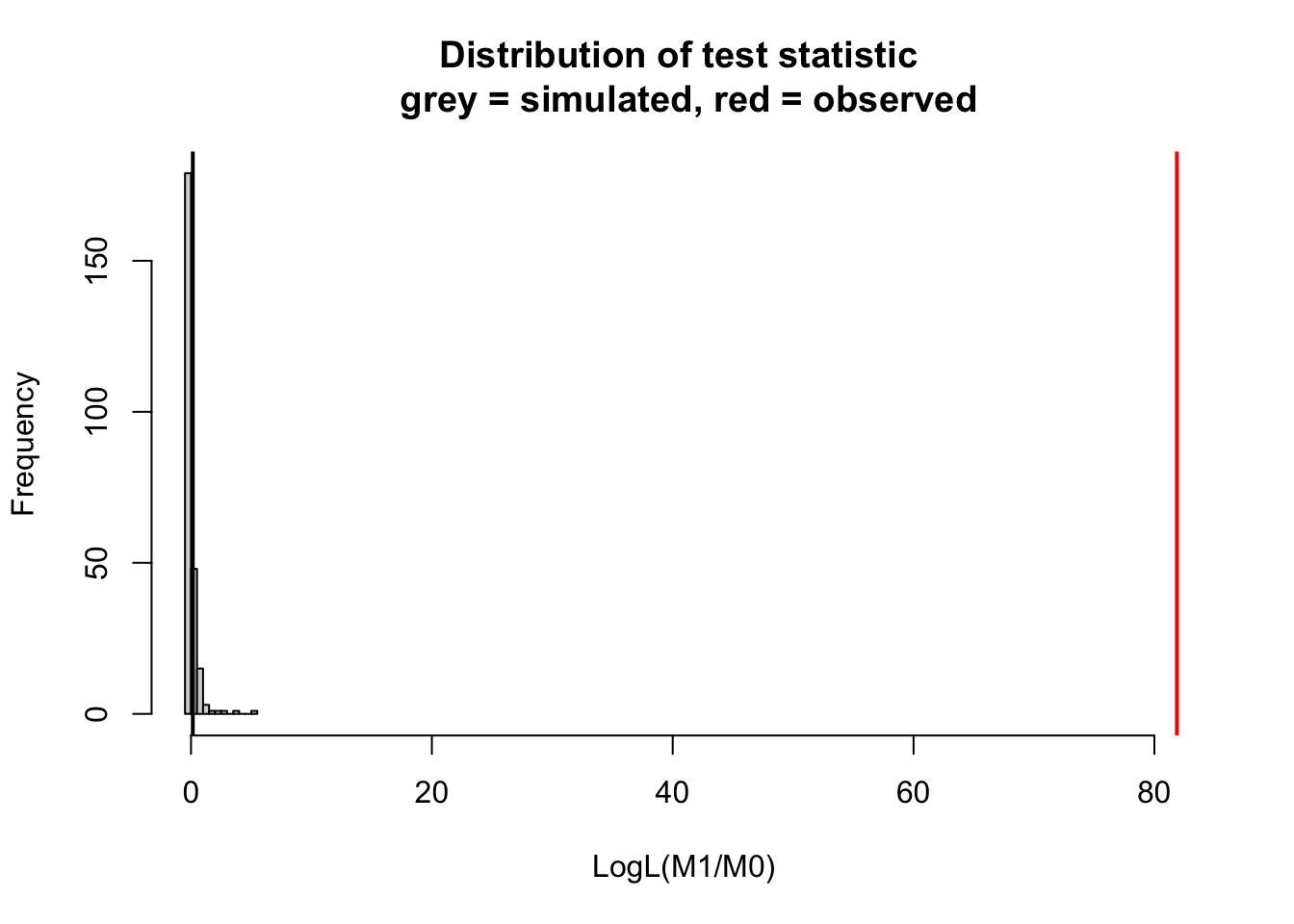


    DHARMa simulated LRT

data:  m0: m0 m1: m1
LogL(M1/M0) = 81.871, p-value < 2.2e-16
alternative hypothesis: M1 describes the data better than M0

If you want to understand the method in more detail, you can expand the hand-coded example of a simulated LRT below:

Hand-coded simulated LRT

We use the models from the previous example - first, let’s look at the observed LR

observedLR = logLik(m1) - logLik(m0)

The log LR of m1 (the RE model) over m0 is 225, meaning that seeing the observed data under m1 is exp(225) times more likely than under m0.

As noted, the complex model will always fit better, so that the data is more likely under M1 is expected, but is the increase significant? In this case, the LR is actually so large that we actually wouldn’t need to test. A rough rule of thumb is that you need a log LR of 2 for each df that you add, and here we have an RE with 10 groups, so even if we could 1 df for each RE group, this should be easily significant. Nevertheless, let’s do the formal test, and this time by hand.

First, we write a function that creates new LRs under H₀, by simulating new data from the fitted M₀, and re-fitting M₀/M₁ to this data, and return the LR.

resampledParameters = function(){
  newData = dat
  newData$observedResponse = unlist(simulate(m0))
  mNew0 = glm(observedResponse ~ Environment1, data = newData, family = "poisson")
  mNew1 = glmer(observedResponse ~ Environment1 + (1|group), data = newData, family = "poisson")
  return(logLik(mNew1) - logLik(mNew0))
}

Now, let’s generate the null distribution. There will be a lot of warnings which you can usually ignore. The reason is that we simulate the data under H₀, i.e. with no RE, and thus the mixed model estimates the RE variance to zero, which creates a warning.

nullDistribution = replicate(500, resampledParameters())

If we plot the null distribution, we see that if the data would really not have an RE, we would expect an increase of likelihood for the more complicated model of not more than 4 or so.

hist(nullDistribution, breaks = 50, main = "Null distribution log(L(M1) / L(M0))")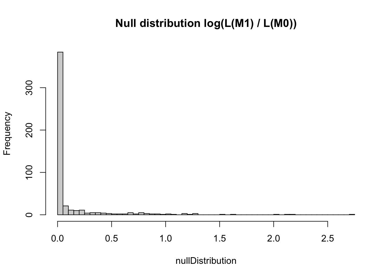

However, what we actually observe is an increase of 225. I rescaled the x axis to make this visible.

hist(nullDistribution, breaks = 50, main = "Null distribution log(L(M1) / L(M0))", xlim = c(-5,250))
abline(v = observedLR, col = "red")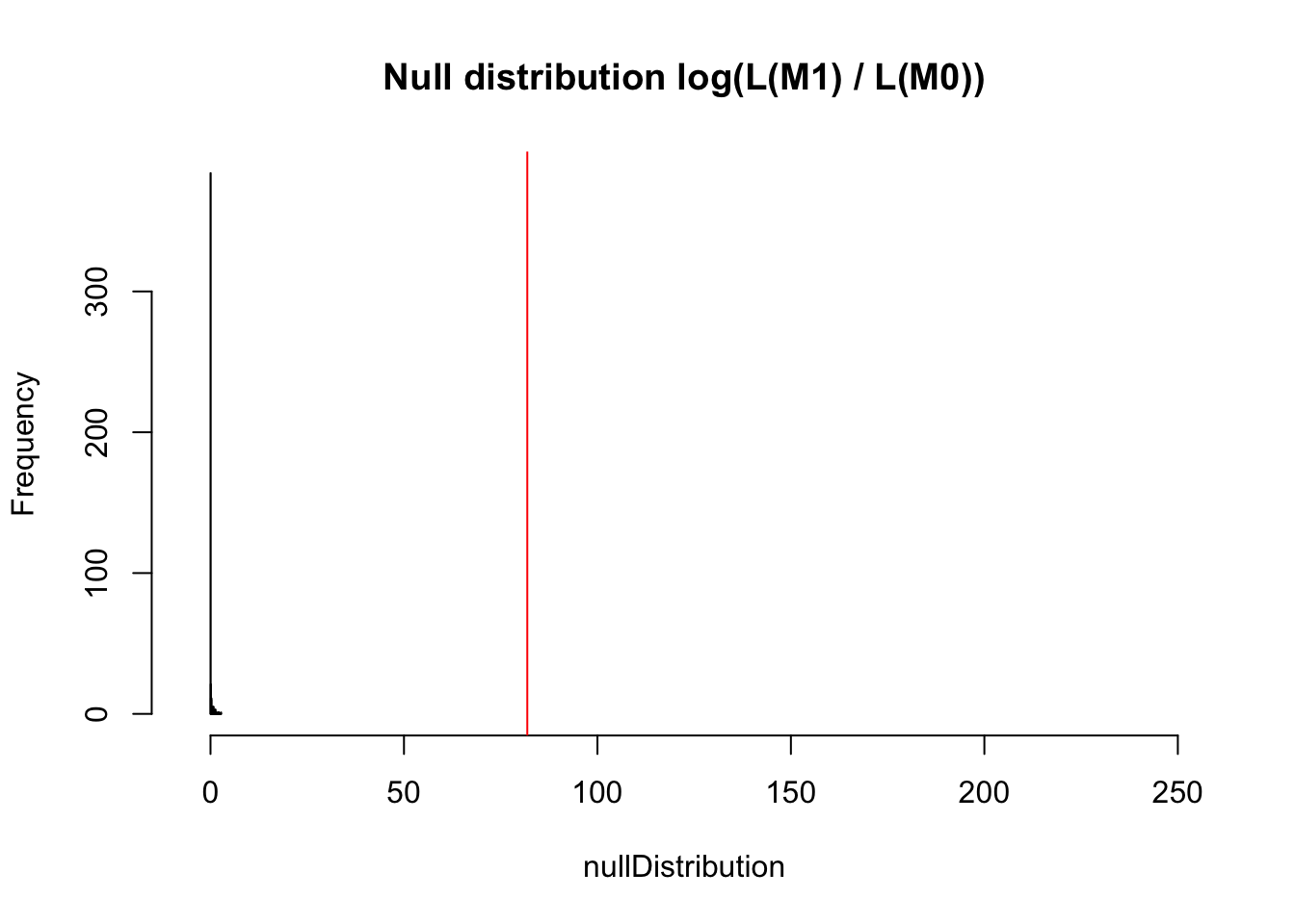

The p-value is 0 obviously

mean(nullDistribution > observedLR)

[1] 0

4.5.4 Variance partitioning / ANOVA

Also variance partitioning in mixed models is a bit tricky, as (see type I/II/III ANOVA discussion) fixed and random components of the model are in some way “correlated”.

First of all, note that you have to be careful because as most S3 functions in R, the anova function is overloaded, so depending on the class of the model object, different functions will be used.

Let’s look at this for the case of a lmer model.

library(faraway)
library(lme4)
detach("package:lmerTest", unload=TRUE)
data(irrigation)
fit <- lmer(yield ~ irrigation + variety + (1|field), data = irrigation)
summary(fit)

Linear mixed model fit by REML ['lmerMod']
Formula: yield ~ irrigation + variety + (1 | field)
   Data: irrigation

REML criterion at convergence: 54.8

Scaled residuals: 
    Min      1Q  Median      3Q     Max 
-0.8751 -0.5615 -0.1090  0.6889  1.0931 

Random effects:
 Groups   Name        Variance Std.Dev.
 field    (Intercept) 16.541   4.067   
 Residual              1.426   1.194   
Number of obs: 16, groups:  field, 8

Fixed effects:
             Estimate Std. Error t value
(Intercept)    38.425      2.952  13.015
irrigationi2    1.000      4.154   0.241
irrigationi3    0.600      4.154   0.144
irrigationi4    4.100      4.154   0.987
varietyv2       0.750      0.597   1.256

Correlation of Fixed Effects:
            (Intr) irrgt2 irrgt3 irrgt4
irrigation2 -0.703                     
irrigation3 -0.703  0.500              
irrigation4 -0.703  0.500  0.500       
varietyv2   -0.101  0.000  0.000  0.000

If you run the anova command on this, it will call anova.merMod from package lme4, which runs a sequential (type I) ANOVA.

anova(fit)

Analysis of Variance Table
           npar Sum Sq Mean Sq F value
irrigation    3 1.6605  0.5535  0.3882
variety       1 2.2500  2.2500  1.5782

See discussions about the exact calculations of this function here.

If you load lmerTest, the anova command will be overwritten by anova.lmerTest, which performs, as displayed in the output, a type III Anova with df estimated by Satterthwaite’s method.

library(lmerTest)
fit <- lmer(yield ~ irrigation + variety + (1|field), data = irrigation)
anova(fit)

Type III Analysis of Variance Table with Satterthwaite's method
           Sum Sq Mean Sq NumDF DenDF F value Pr(>F)
irrigation 1.6605  0.5535     3     4  0.3882 0.7685
variety    2.2500  2.2500     1     7  1.5782 0.2493

Arguably, this method is preferable over the based lme4 method if you are interested in the p-values of the model terms.

Another common question in ANOVA for mixed models is how much R2 is explained by fixed vs. random effects. Philosophically, the main point of discussion here is: Do you want to count the random effect variance as “explained”, or “residual”. In any case, aommon approach is the hierarchical partitioning proposed by by Nakagawa & Schielzeth 2013, Nakagawa et al. (2017), which is implemented in the MuMIn package. With this, we can run

library(MuMIn)
r.squaredGLMM(fit)

           R2m       R2c
[1,] 0.1360522 0.9314427

Interpretation

R²m: Marginal R² value associated with fixed effects.
R²c: Conditional R² value associated with fixed effects plus the random effects.

It is important to note that this is a description of the fitted model, not necessarily valid inference - the reason is that if you add a lot of REs, you will tend to get a lot of variance explained by the RE structure. If you want to correct for this, one option is to calculate R² values under a cross-validation.

4.5.5 Variance partition coefficients (VPCs)

An interesting variation of using mixed models is to use them as an alternative to ANOVA to understand how much variation in a response variable is explained by different factor variables (for applications in ecology, see (Leite et al. 2024)). Consider the following example of simulated data, where I created 3 categorical variables with an increasing number of levels per variable, and essentially a “normal” distribution of effects for the different levels of those. In other words, these are exactly the assumptions of a mixed model, where we have 4 normally distributed errors: 3 for the 3 groups (with different group sizes) and 1 residual error, all with the same sd of 1.

set.seed(123)

k1 = 4
k2 = 8
k3 = 20
rep = 5

RE1 = rnorm(k1)
RE2 = rnorm(k2)
RE3 = rnorm(k3)

dat = expand.grid(1:k1,1:k2,1:k3, 1:rep)
dat$y = RE1[dat$Var1] + RE2[dat$Var2] + RE3[dat$Var3] + rnorm(nrow(dat))
dat[1:4] <- lapply(dat[1:4], as.factor)

To see how much variation is created by each of the factors, the standard way would be to fit an ANOVA (see section on ANOVA if you don’t recall the details). As the design is perfectly balanced and orthogonal, it doesn’t matter if we fit type I,II,III ANOVA:

summary(aov(y ~ Var1+Var2+Var3, data = dat))

              Df Sum Sq Mean Sq F value Pr(>F)    
Var1           3   2116   705.3   713.0 <2e-16 ***
Var2           7   2726   389.5   393.8 <2e-16 ***
Var3          19   2650   139.5   141.0 <2e-16 ***
Residuals   3170   3136     1.0                   
---
Signif. codes:  0 '***' 0.001 '**' 0.01 '*' 0.05 '.' 0.1 ' ' 1

# car::Anova(lm(y ~ Var1+Var2+Var3, data = dat)) # identical

The alternative would be to fit a random effect model with the 3 grouping variables as random intercepts

library(lme4)
library(lmerTest)
fit <- lmer(y ~ (1|Var1) + (1|Var2) + (1|Var3), data = dat)

After having fit the model, we can look at the the random effect table

x = VarCorr(fit)
x

 Groups   Name        Std.Dev.
 Var3     (Intercept) 0.93045 
 Var2     (Intercept) 0.98556 
 Var1     (Intercept) 0.93829 
 Residual             0.99458

Which pretty much already looks like an ANOVA table. If you standardize the RE variances to sum of all variance, you obtain the so-called variance partition coefficients (VPCs)., which are often seen as an alternative to ANOVA

x = data.frame(x)
x$vcov / sum(x$vcov)

[1] 0.2335613 0.2620508 0.2375173 0.2668705

Important

Note that the results of a VPC can be very different from an ANOVA. In an ANOVA, you look at the variance explained in the response. In VPCs, you compare the the variance between different groups in the data. This will tend to be similar to ANOVA if ob observations are balanced in groups, but it can be very different if they are not. In this behavior, VPCs resemble standardized effect sizes (which can also differ in ranking variables from ANOVA if the distribution of the predictor is very skewed). I would therefore recommend to interpret VPCs as “effect sizes of categorical predictors”, rather than as ANOVA shares.

We can get (note: approximate) p-values on the terms by running a random effect anova

lmerTest::ranova(fit)

ANOVA-like table for random-effects: Single term deletions

Model:
y ~ (1 | Var1) + (1 | Var2) + (1 | Var3)
           npar  logLik     AIC    LRT Df Pr(>Chisq)    
<none>        5 -4603.6  9217.3                         
(1 | Var1)    4 -5410.4 10828.7 1613.5  1  < 2.2e-16 ***
(1 | Var2)    4 -5573.1 11154.2 1938.9  1  < 2.2e-16 ***
(1 | Var3)    4 -5523.9 11055.8 1840.6  1  < 2.2e-16 ***
---
Signif. codes:  0 '***' 0.001 '**' 0.01 '*' 0.05 '.' 0.1 ' ' 1

The quality of the p-value approximation is somewhat unclear. Alternatively, you could run non-parametric simulation-based LRTs (see section on testing on the RE structure). In a frequentist framework, it will be difficult to obtain CIs on the VPCs, unless you bootstrap. Alternatively, you could run this in a Bayesian framework via brms.

As a final step, let’s test out if we test for factors that did not have an effect in the model. In this case, I create a 3 two-way interaction as well as another RE on the factor replicate, which did not have an effect on the response

dat$Var12 = factor(paste(dat$Var1,dat$Var2))
dat$Var23 = factor(paste(dat$Var2,dat$Var3))
dat$Var13 = factor(paste(dat$Var1,dat$Var3))

summary(aov(y ~ (Var1+Var2+Var3)^2 +Var4, data = dat))

              Df Sum Sq Mean Sq F value Pr(>F)    
Var1           3 2115.8   705.3 712.057 <2e-16 ***
Var2           7 2726.5   389.5 393.253 <2e-16 ***
Var3          19 2650.5   139.5 140.844 <2e-16 ***
Var4           4    2.4     0.6   0.601 0.6623    
Var1:Var2     21   33.1     1.6   1.592 0.0424 *  
Var1:Var3     57   56.3     1.0   0.997 0.4814    
Var2:Var3    133  117.1     0.9   0.889 0.8115    
Residuals   2955 2926.8     1.0                   
---
Signif. codes:  0 '***' 0.001 '**' 0.01 '*' 0.05 '.' 0.1 ' ' 1

fit <- lmer(y ~ (1|Var1) + (1|Var2) + (1|Var3) + (1|Var12) +  + (1|Var23) + (1|Var13) +  (1|Var4)  , data = dat)
VarCorr(fit)

 Groups   Name        Std.Dev. 
 Var23    (Intercept) 0.0000000
 Var13    (Intercept) 0.0083897
 Var12    (Intercept) 0.0769290
 Var3     (Intercept) 0.9305624
 Var2     (Intercept) 0.9849222
 Var4     (Intercept) 0.0000000
 Var1     (Intercept) 0.9382560
 Residual             0.9925834

lmerTest::ranova(fit)

ANOVA-like table for random-effects: Single term deletions

Model:
y ~ (1 | Var1) + (1 | Var2) + (1 | Var3) + (1 | Var12) + (1 | Var23) + (1 | Var13) + (1 | Var4)
            npar  logLik    AIC     LRT Df Pr(>Chisq)    
<none>         9 -4602.3 9222.5                          
(1 | Var1)     8 -4641.6 9299.2  78.627  1    < 2e-16 ***
(1 | Var2)     8 -4640.9 9297.8  77.216  1    < 2e-16 ***
(1 | Var3)     8 -4691.5 9399.0 178.407  1    < 2e-16 ***
(1 | Var12)    8 -4603.6 9223.3   2.711  1    0.09965 .  
(1 | Var23)    8 -4602.3 9220.5   0.001  1    0.97069    
(1 | Var13)    8 -4602.3 9220.5   0.000  1    0.98888    
(1 | Var4)     8 -4602.3 9220.5   0.000  1    1.00000    
---
Signif. codes:  0 '***' 0.001 '**' 0.01 '*' 0.05 '.' 0.1 ' ' 1

In this case, both methods attribute some variation to the null terms, but also both methods realize that these terms are (mostly) n.s., which is re-assuring! Ther term V12 is around 0.05, significant in ANOVA and n.s. in VPC, suggesting maybe that the VPC could be a bit more conservative, although I suspect that this is highly context and package dependent (as different packages fit the REs differently). Note that I have surpressed boundary / convergence warnings in the fit of the mixed model, which should be of course solved in a real application.

VPC vs. ANOVA

So, when and why should you prefer VPC over ANOVA?

A considerable advantage of the VPCs over ANOVA is that they compute orders of magnitudes faster than a standard anova in large datasets with many group levels.

Disadvantages are measures of uncertainty (p-values, CIs) may be problematic to obtain. Moreover, you should also note that the estimation of the VPCs depends on the ability of the mixed models to estimate the correct RE variance. To obtain unbiased estimates of the RE variance is notoriously difficult, as evidenced by the different methods to estimate the RE variances in different packages, as well as the REML / ML estimation debate (see section on REML). The issues are usually not a primary concern, because we usually do not interpret the RE variances directly, but they are only indirectly used to account for the group level effects. In the VPC analysis, however, they are directly used, and thus particular care should be taken, e.g., in checking if RE distributions are indeed normal etc. (see, e.g., section on residual checks for mixed models).

4.6 Case studies

4.6.1 Honeybee Data

We use a dataset on bee colonies infected by the American Foulbrood (AFB) disease. The study measured spores of the bacterium “Paenibacillus larvae” (variable Spobee) that infect honeybee larvae, as well as the degree of the infection of the colony (integer: 0 (none), 1 (minor), 2 (moderate), 3 (major)).

The scientific question is if colonies with a higher degree of infection also exhibit more spores, i.e. if infection predicts spores. Additional variables that you can consider are BeesN (Bees per hive) and Hive (ID of the respective hive. (integer, 1 - 24).)

Task: fit an appropriate linear mixed model on this data.

library(EcoData)
str(bees)

'data.frame':   72 obs. of  6 variables:
 $ Spobee   : num  6.67 13.33 6.67 6.67 20 ...
 $ Hive     : int  1 1 1 2 2 2 3 3 3 4 ...
 $ X        : int  0 0 0 0 0 0 0 0 0 0 ...
 $ Y        : num  0 0 0 91 91 91 262 262 262 353 ...
 $ Infection: int  0 0 0 0 0 0 0 0 0 0 ...
 $ BeesN    : int  95000 95000 95000 95000 95000 95000 85000 85000 85000 90000 ...

Perform the data analysis, according to the hypothesis discussed in the course.

Solution

Because of the skewed distribution of Spobee, it is better to use log(Spobee + 1) or something similar as response (else you will not get nice residuals)
I decided to add BeesN in the regression because it could be a confounder (more on confounding in section on causal inference)
It is natural to model hive as a random intercept (1|Hive). I don’t expect that the infection ~ spores relationship should be different between hives, but can test for this after fitting the model

library(lme4)
fit <- lmer(log(Spobee + 1) ~ Infection + BeesN + (1|Hive), data = bees)
summary(fit)

Linear mixed model fit by REML. t-tests use Satterthwaite's method [
lmerModLmerTest]
Formula: log(Spobee + 1) ~ Infection + BeesN + (1 | Hive)
   Data: bees

REML criterion at convergence: 260.8

Scaled residuals: 
     Min       1Q   Median       3Q      Max 
-2.27939 -0.45413  0.09209  0.52159  1.64023 

Random effects:
 Groups   Name        Variance Std.Dev.
 Hive     (Intercept) 4.8463   2.2014  
 Residual             0.6033   0.7767  
Number of obs: 72, groups:  Hive, 24

Fixed effects:
              Estimate Std. Error         df t value Pr(>|t|)    
(Intercept)  5.583e+00  1.907e+00  2.100e+01   2.927  0.00805 ** 
Infection    2.663e+00  5.528e-01  2.100e+01   4.818 9.22e-05 ***
BeesN       -2.068e-05  2.558e-05  2.100e+01  -0.808  0.42804    
---
Signif. codes:  0 '***' 0.001 '**' 0.01 '*' 0.05 '.' 0.1 ' ' 1

Correlation of Fixed Effects:
          (Intr) Infctn
Infection -0.476       
BeesN     -0.966  0.398
fit warnings:
Some predictor variables are on very different scales: consider rescaling

Standard residual plots look fine, possible minor evidence for heteroskedasticity

plot(fit)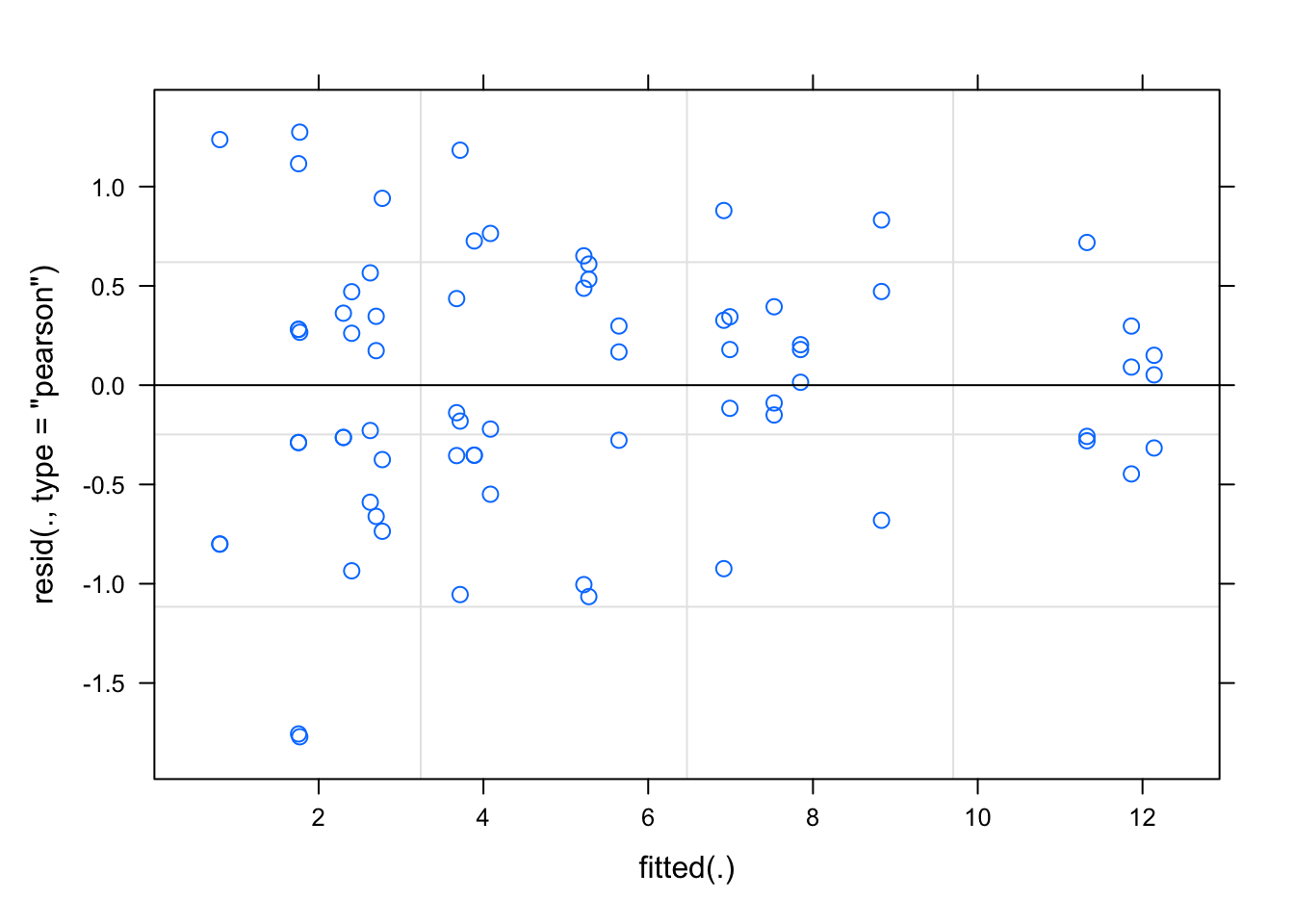

Let’s have a look at the random effects

x = ranef(fit)
qqnorm(x$Hive$`(Intercept)`)
qqline(x$Hive$`(Intercept)`)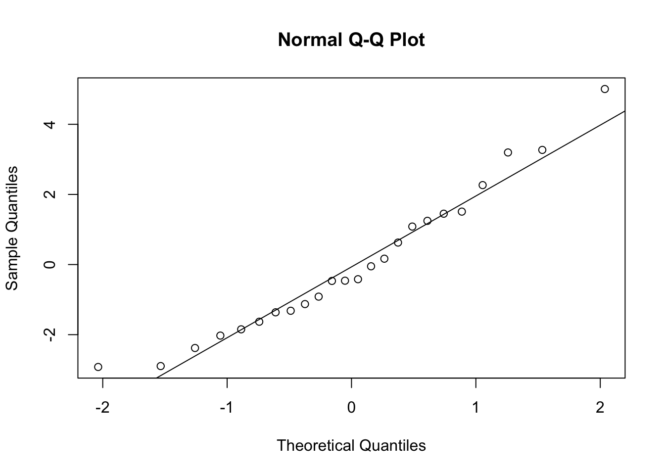

shapiro.test(x$Hive$`(Intercept)`)


    Shapiro-Wilk normality test

data:  x$Hive$`(Intercept)`
W = 0.95543, p-value = 0.3537

Looks good. Could also check with DHARMa. The default plot calculates residuals, i.e. residuals based on random effect and residual variation together. This leads to more noise, which, however, I would disregard in this case.

simulateResiduals(fit, plot = T)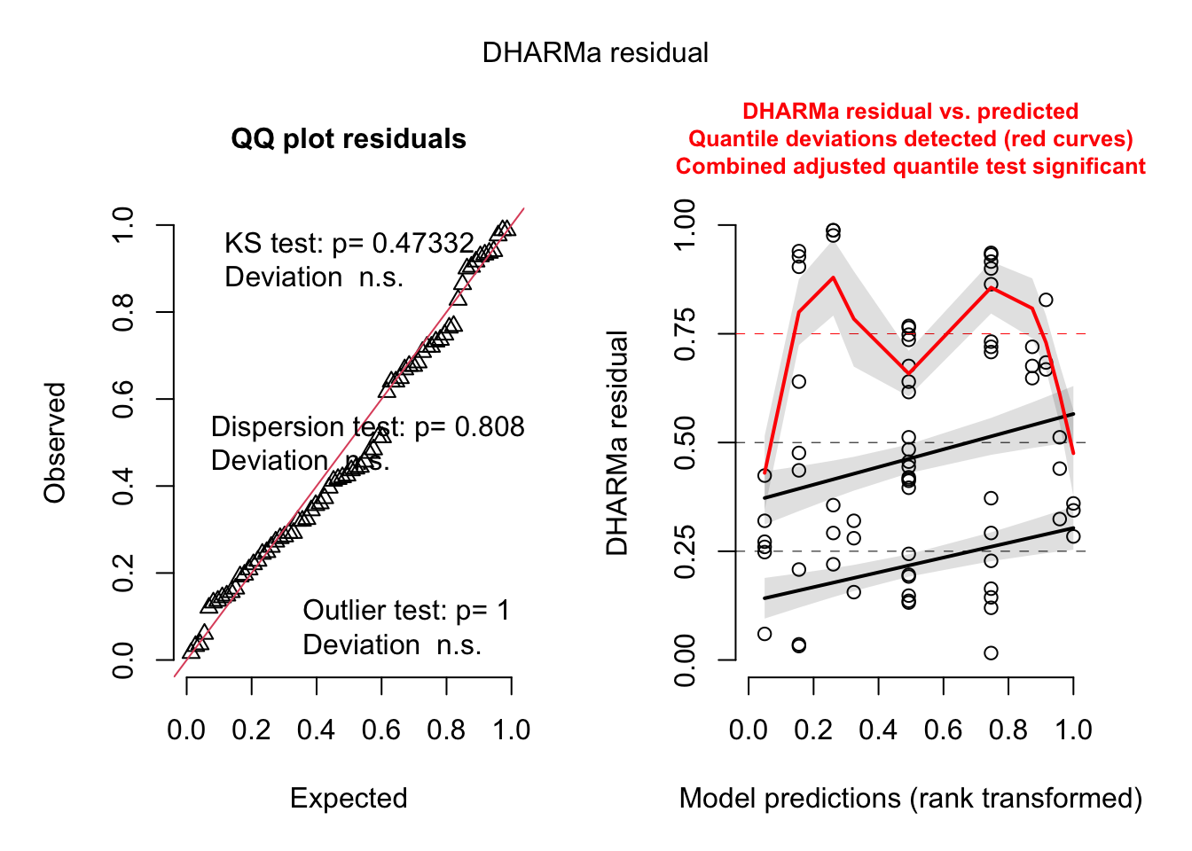

Object of Class DHARMa with simulated residuals based on 250 simulations with refit = FALSE . See ?DHARMa::simulateResiduals for help. 
 
Scaled residual values: 0.272 0.32 0.26 0.248 0.424 0.06 0.356 0.22 0.292 0.476 0.436 0.64 0.208 0.036 0.032 0.988 0.988 0.976 0.016 0.228 ...

With lme4, you can switch to conditinal residuals by using the re.form syntax of lme4

simulateResiduals(fit, plot = T, re.form = NULL)

Object of Class DHARMa with simulated residuals based on 250 simulations with refit = FALSE . See ?DHARMa::simulateResiduals for help. 
 
Scaled residual values: 0.388 0.672 0.372 0.624 0.96 0.008 0.688 0.192 0.568 0.364 0.32 0.84 0.948 0.208 0.12 0.864 0.732 0.192 0.02 0.944 ...

Residual plot to check for evidence of a random slope shows that hives are either infected or not, thus doesn’t make sense to add a random slope

plot(fit, 
     resid(., scaled=TRUE) ~ fitted(.) | Hive, 
     abline = 0)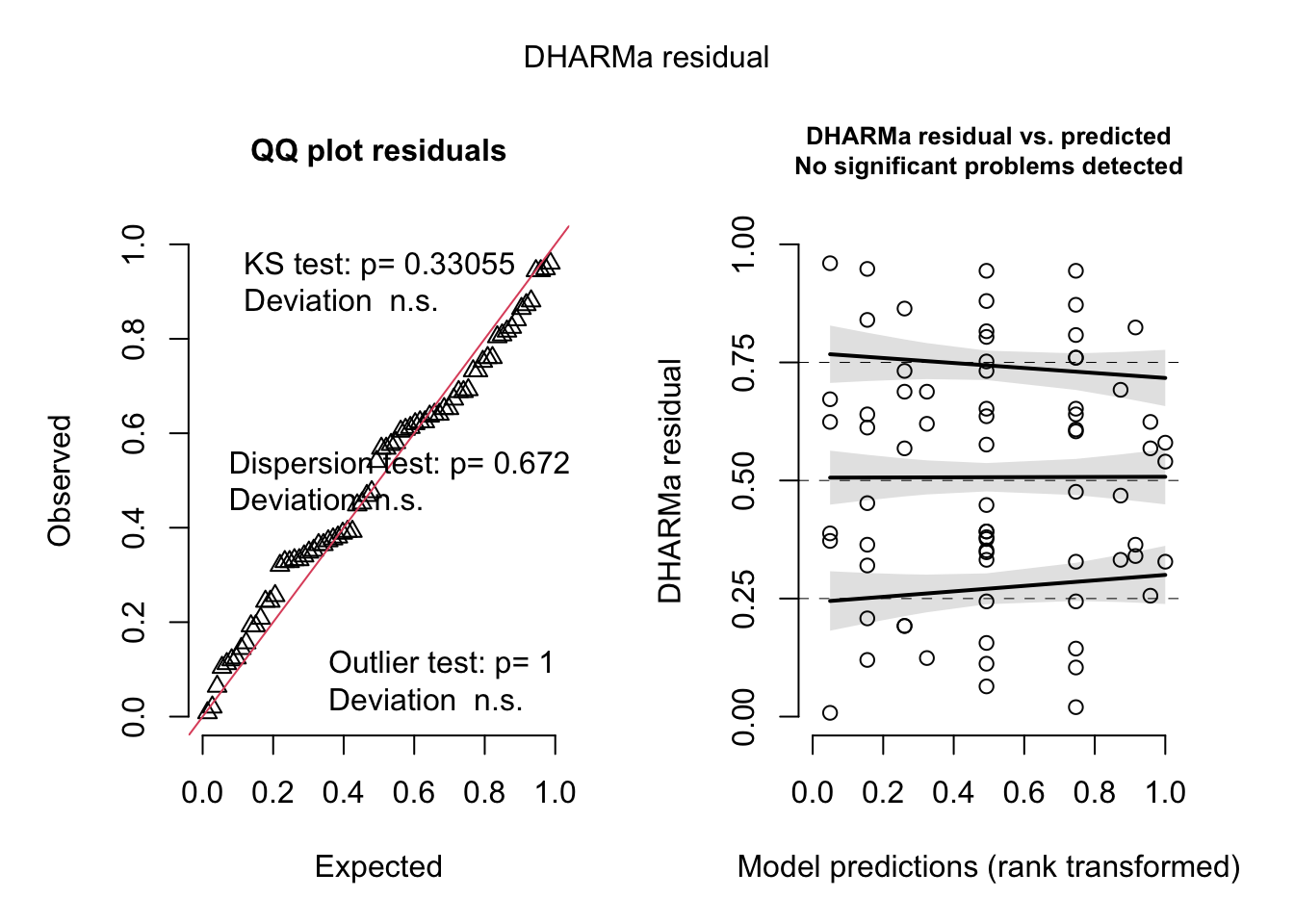

4.6.2 College Student Performance

The GPA (college grade point average) data is a longitudinal data set (also named panel data, German: “Längsschnittstudie”. A study repeated at several different moments in time, compared to a cross-sectional study (German: “Querschnittstudie”) which has several participants at one time). In this data set, 200 college students and their GPA have been followed 6 consecutive semesters. Look at the GPA data set, which can be found in the EcoData package:

library(EcoData)
str(gpa)

In this data set, there are GPA measures on 6 consecutive occasions, with a job status variable (how many hours worked) for the same 6 occasions. There are two student-level explanatory variables: The sex (1 = male, 2 = female) and the high school gpa. There is also a dichotomous student-level outcome variable, which indicates whether a student has been admitted to the university of their choice. Since not every student applies to a university, this variable has many missing values. Each student and each year of observation have an id.

Task

Analyze if the student’s GPA improves over time (occasion)! Here a few hints to look at:

Consider which fixed effect structure you want to fit. For example, you might be interested if males and females differ in their temporal trend
Student is the grouping variable -> RE. Which RE structure do you want to fit? A residual plot may help
For your benefit, have a look at the difference in the regression table (confidence intervals, coefficients and p-values) of mixed and corresponding fixed effects model. You can also look at the estimates of the mixed effects model (hint: ?ranef).
After having specified the mixed model, have a look at residuals.

Solution

library(lme4)
library(glmmTMB)
library(EcoData)
# initial model with a random intercept and fixed effect structure based on
# causal assumptions

gpa$sOccasion = scale(gpa$occasion)
gpa$nJob = as.numeric(gpa$job)

fit <- lmer(gpa ~ sOccasion*sex + nJob + (1|student), data = gpa)
summary(fit)

# plot seems to show a lot of differences still, so add random slope
plot(fit, 
     resid(., scaled=TRUE) ~ fitted(.) | student, 
     abline = 0)

# slope + intercept model
fit <- lmer(gpa ~ sOccasion*sex + nJob + (sOccasion|student), data = gpa)

# checking residuals - heteroskedasticity 
plot(fit)

# We only learn later how to specify a variable, dispersion, but as a teaser - I'm modelling this using glmmTMB, alternatively could add weights nlme::lme, which also allows specifying mixed models with all variance modelling options that we discussed for gls, but random effect specification is different than here
fit <- glmmTMB(gpa ~ sOccasion*sex + nJob + (sOccasion|student), data = gpa, dispformula = ~ sOccasion)
summary(fit)

# unfortunately, the dispersion in this model cannot be reliably checked, because the functions for this are not (yet) implemented in glmmTMB
plot(residuals(fit, type = "pearson") ~ predict(fit)) # not implemented
library(DHARMa)
simulateResiduals(fit, plot = T) 
# still, the variable dispersion model is highly supported by the data and clearly preferable over a fixed dispersion model