Appendix C — Case studies

Appendix C — Case studies

General strategy for analysis:

Define formula via scientific questions + confounders.
Define type of GLM (lm, logistic, Poisson).
Blocks in data -> Random effects, start with random intercept.

Fit this base model, then do residual checks for

Wrong functional form -> Change fitted function.
Wrong distribution-> Transformation or GLM adjustment.
(Over)dispersion -> Variable dispersion GLM.
Heteroskedasticity -> Model dispersion.
Zero-inflation -> Add ZIP term.
…

And adjust the model accordingly.

C.1 Hurricanes

In https://www.pnas.org/content/111/24/8782, Jung et al. claim that “Female hurricanes are deadlier than male hurricanes”.

Specifically, they analyze the number of hurricane fatalities, and claim that there is an effect of the femininity of the name on the number of fatalities, correcting for several possible confounders. They interpret the result as causal (including mediators), claiming that giving only male names to hurricanes would considerably reduce death toll.

The data is available in DHARMa.

library(DHARMa)
library(mgcv)
?hurricanes
str(hurricanes)

Classes 'tbl_df', 'tbl' and 'data.frame':   92 obs. of  14 variables:
 $ Year                    : num  1950 1950 1952 1953 1953 ...
 $ Name                    : chr  "Easy" "King" "Able" "Barbara" ...
 $ MasFem                  : num  6.78 1.39 3.83 9.83 8.33 ...
 $ MinPressure_before      : num  958 955 985 987 985 960 954 938 962 987 ...
 $ Minpressure_Updated_2014: num  960 955 985 987 985 960 954 938 962 987 ...
 $ Gender_MF               : num  1 0 0 1 1 1 1 1 1 1 ...
 $ Category                : num  3 3 1 1 1 3 3 4 3 1 ...
 $ alldeaths               : num  2 4 3 1 0 60 20 20 0 200 ...
 $ NDAM                    : num  1590 5350 150 58 15 ...
 $ Elapsed_Yrs             : num  63 63 61 60 60 59 59 59 58 58 ...
 $ Source                  : chr  "MWR" "MWR" "MWR" "MWR" ...
 $ ZMasFem                 : num  -0.000935 -1.670758 -0.913313 0.945871 0.481075 ...
 $ ZMinPressure_A          : num  -0.356 -0.511 1.038 1.141 1.038 ...
 $ ZNDAM                   : num  -0.439 -0.148 -0.55 -0.558 -0.561 ...

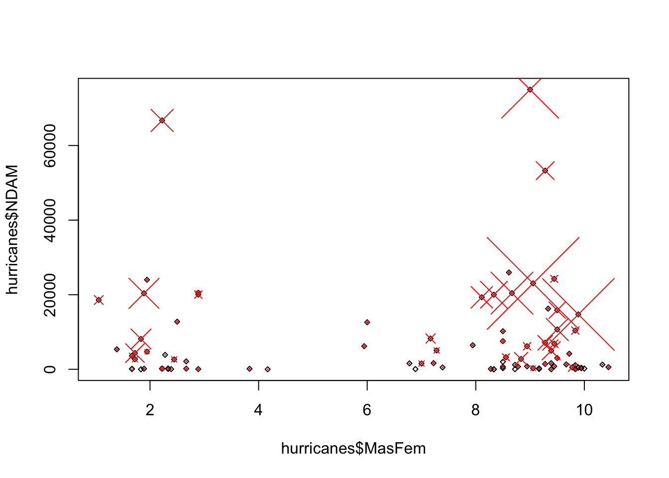
Some plots:

plot(hurricanes$MasFem, hurricanes$NDAM, cex = 0.5, pch = 5)
points(hurricanes$MasFem, hurricanes$NDAM, cex = hurricanes$alldeaths/20,
       pch = 4, col= "red")

The original model from the paper fits a negative binomial, using mgcv.{R}. I suppose the reason is mainly that glmmTMB was not available at the time, and implementations of the negative binomial, in particular mass::glm.nb and lme4::glmer.nb often had convergence problems.

originalModelGAM = gam(alldeaths ~ MasFem * (Minpressure_Updated_2014 + NDAM),
    data = hurricanes, family = nb, na.action = "na.fail")
summary(originalModelGAM)


Family: Negative Binomial(0.736) 
Link function: log 

Formula:
alldeaths ~ MasFem * (Minpressure_Updated_2014 + NDAM)

Parametric coefficients:
                                  Estimate Std. Error z value Pr(>|z|)    
(Intercept)                      7.014e+01  2.003e+01   3.502 0.000462 ***
MasFem                          -5.986e+00  2.529e+00  -2.367 0.017927 *  
Minpressure_Updated_2014        -7.008e-02  2.060e-02  -3.402 0.000669 ***
NDAM                            -3.845e-05  2.945e-05  -1.305 0.191735    
MasFem:Minpressure_Updated_2014  6.124e-03  2.603e-03   2.352 0.018656 *  
MasFem:NDAM                      1.593e-05  3.756e-06   4.242 2.21e-05 ***
---
Signif. codes:  0 '***' 0.001 '**' 0.01 '*' 0.05 '.' 0.1 ' ' 1


R-sq.(adj) =  -3.61e+03   Deviance explained = 57.4%
-REML = 357.56  Scale est. = 1         n = 92

Caution

Tasks:

Confirm that you get the same results as in the paper. It makes sense to translate their model to glmmTMB. Note that the nb parameterization of mgcv corresponds to nbinom2 in glmmTMB. You will get different results when choosing nbinom1
Inspect the fitted model for potential problems, in particular perform a residual analysis of the model, including residuals against all predictors, and improve the model if you find problems.
Forget what they did. Go back to start, do a causal analysis like we did, and do your own model, diagnosing all residual problems that we discussed. Do you think there is an effect of femininity?

Solution

This is the model fit by Jung et al., fit with glmmTMB

library(DHARMa)
library(glmmTMB)

m1 = glmmTMB(alldeaths ~ MasFem*
                             (Minpressure_Updated_2014 + scale(NDAM)),
                           data = hurricanes, family = nbinom2)
summary(m1)

 Family: nbinom2  ( log )
Formula:          alldeaths ~ MasFem * (Minpressure_Updated_2014 + scale(NDAM))
Data: hurricanes

     AIC      BIC   logLik deviance df.resid 
   660.7    678.4   -323.4    646.7       85 


Dispersion parameter for nbinom2 family (): 0.787 

Conditional model:
                                 Estimate Std. Error z value Pr(>|z|)    
(Intercept)                     69.661590  23.425598   2.974 0.002942 ** 
MasFem                          -5.855078   2.716589  -2.155 0.031138 *  
Minpressure_Updated_2014        -0.069870   0.024251  -2.881 0.003964 ** 
scale(NDAM)                     -0.494094   0.455968  -1.084 0.278536    
MasFem:Minpressure_Updated_2014  0.006108   0.002813   2.171 0.029901 *  
MasFem:scale(NDAM)               0.205418   0.061956   3.316 0.000915 ***
---
Signif. codes:  0 '***' 0.001 '**' 0.01 '*' 0.05 '.' 0.1 ' ' 1

Note that in the code that I gave you not all predictors were scaled (and they don’t say if they scaled in the paper), but as we for looking for main effects in the presence of interactions, we should definitely scale to improve the interpretability

m2 = glmmTMB(alldeaths ~ scale(MasFem) *
                             (scale(Minpressure_Updated_2014) + scale(NDAM)),
                           data = hurricanes, family = nbinom2)
summary(m2)

 Family: nbinom2  ( log )
Formula:          
alldeaths ~ scale(MasFem) * (scale(Minpressure_Updated_2014) +  
    scale(NDAM))
Data: hurricanes

     AIC      BIC   logLik deviance df.resid 
   660.7    678.4   -323.4    646.7       85 


Dispersion parameter for nbinom2 family (): 0.787 

Conditional model:
                                              Estimate Std. Error z value
(Intercept)                                     2.5034     0.1231  20.341
scale(MasFem)                                   0.1237     0.1210   1.022
scale(Minpressure_Updated_2014)                -0.5425     0.1603  -3.384
scale(NDAM)                                     0.8988     0.2190   4.105
scale(MasFem):scale(Minpressure_Updated_2014)   0.3758     0.1731   2.171
scale(MasFem):scale(NDAM)                       0.6629     0.1999   3.316
                                              Pr(>|z|)    
(Intercept)                                    < 2e-16 ***
scale(MasFem)                                 0.306923    
scale(Minpressure_Updated_2014)               0.000715 ***
scale(NDAM)                                   4.05e-05 ***
scale(MasFem):scale(Minpressure_Updated_2014) 0.029901 *  
scale(MasFem):scale(NDAM)                     0.000915 ***
---
Signif. codes:  0 '***' 0.001 '**' 0.01 '*' 0.05 '.' 0.1 ' ' 1

now main effect is n.s.; it’s a bit dodgy, but if you read in the main paper, they do not claim a significant main effect, they mainly argue via ANOVA and significance at high values of NDAM, so let’s run an ANOVA:

car::Anova(m2)

Analysis of Deviance Table (Type II Wald chisquare tests)

Response: alldeaths
                                                Chisq Df Pr(>Chisq)    
scale(MasFem)                                  1.9495  1  0.1626364    
scale(Minpressure_Updated_2014)                7.1285  1  0.0075868 ** 
scale(NDAM)                                   14.6100  1  0.0001322 ***
scale(MasFem):scale(Minpressure_Updated_2014)  4.7150  1  0.0299011 *  
scale(MasFem):scale(NDAM)                     10.9929  1  0.0009146 ***
---
Signif. codes:  0 '***' 0.001 '**' 0.01 '*' 0.05 '.' 0.1 ' ' 1

In the ANOVA we see that MasFem still n.s. but interactions, and if you would calculate effect of MasFem at high NDAM, it is significant. Something like that is argued in the paper. We can emulate this by changing NDAM centering to high NDAM, which gives us a p-value for the main effect of MasFem at high values of NDAM

hurricanes$highcenteredNDAM = hurricanes$NDAM - max(hurricanes$NDAM)

m3 = glmmTMB(alldeaths ~ scale(MasFem) *
                             (scale(Minpressure_Updated_2014) + highcenteredNDAM),
                           data = hurricanes, family = nbinom2)
summary(m3)

 Family: nbinom2  ( log )
Formula:          
alldeaths ~ scale(MasFem) * (scale(Minpressure_Updated_2014) +  
    highcenteredNDAM)
Data: hurricanes

     AIC      BIC   logLik deviance df.resid 
   660.7    678.4   -323.4    646.7       85 


Dispersion parameter for nbinom2 family (): 0.787 

Conditional model:
                                                Estimate Std. Error z value
(Intercept)                                    7.210e+00  1.149e+00   6.275
scale(MasFem)                                  3.595e+00  1.041e+00   3.455
scale(Minpressure_Updated_2014)               -5.425e-01  1.603e-01  -3.384
highcenteredNDAM                               6.949e-05  1.693e-05   4.105
scale(MasFem):scale(Minpressure_Updated_2014)  3.758e-01  1.731e-01   2.171
scale(MasFem):highcenteredNDAM                 5.125e-05  1.546e-05   3.316
                                              Pr(>|z|)    
(Intercept)                                   3.50e-10 ***
scale(MasFem)                                 0.000551 ***
scale(Minpressure_Updated_2014)               0.000715 ***
highcenteredNDAM                              4.05e-05 ***
scale(MasFem):scale(Minpressure_Updated_2014) 0.029904 *  
scale(MasFem):highcenteredNDAM                0.000915 ***
---
Signif. codes:  0 '***' 0.001 '**' 0.01 '*' 0.05 '.' 0.1 ' ' 1

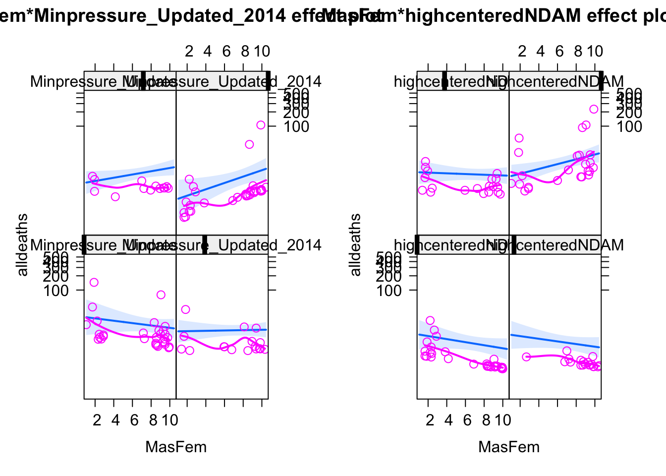
Now we see the significant main effect that they report. Note, hwoever, that the signficant differences is only there for high NDAM, i.e. what we do here is to project the effect of the interaction on the main effect. An alternative to do the same thing would be an effects plot, or to specifically use predict() to calculate differences and CIs at high NDAM values.

library(effects)

Loading required package: carData

lattice theme set by effectsTheme()
See ?effectsTheme for details.

plot(allEffects(m3, partial.residuals = T))

Warning in Effect.glmmTMB(predictors, mod, vcov. = vcov., ...): overriding
variance function for effects/dev.resids: computed variances may be incorrect

Warning in Analyze.model(focal.predictors, mod, xlevels, default.levels, :
the predictors scale(MasFem), scale(Minpressure_Updated_2014) are one-column
matrices that were converted to vectors

Warning in Effect.glmmTMB(predictors, mod, vcov. = vcov., ...): overriding
variance function for effects/dev.resids: computed variances may be incorrect

Warning in Analyze.model(focal.predictors, mod, xlevels, default.levels, :
the predictors scale(MasFem), scale(Minpressure_Updated_2014) are one-column
matrices that were converted to vectors

OK, this means we can replicate the results of the paper, even if concentrating the entire analysis exclusive on high NDAM seems a bit cherry-picking. Another way to phrase the result is that we don’t find a main effect of MasFem. However, to be fair: the current results to say that there is a significant difference at high NDAM, and such a difference, if it existed, would be importat.

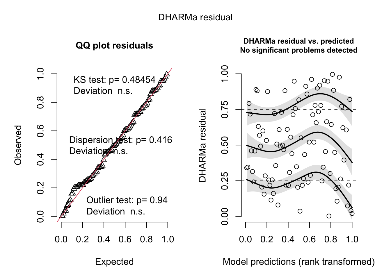
But we haven’t done residual checks yet. Let’s do that:

res <- simulateResiduals(originalModelGAM)

Registered S3 method overwritten by 'GGally':
  method from   
  +.gg   ggplot2

Registered S3 method overwritten by 'mgcViz':
  method from  
  +.gg   GGally

plot(res)

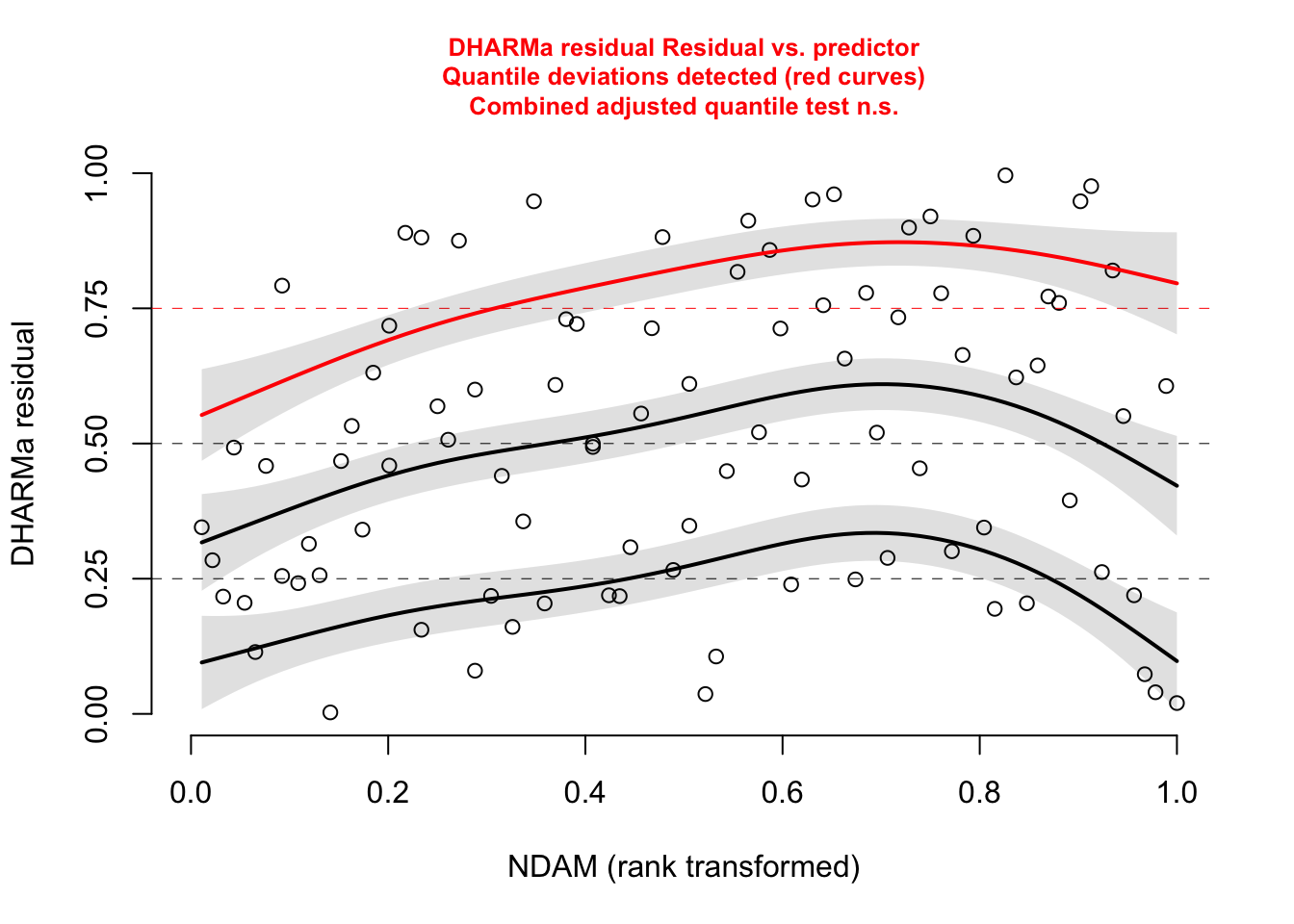
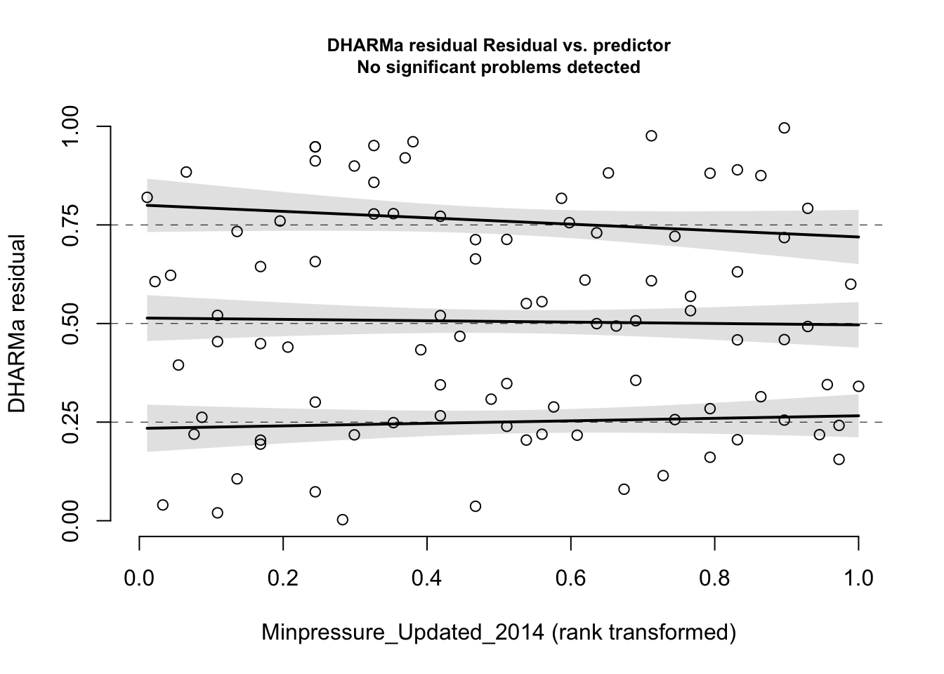
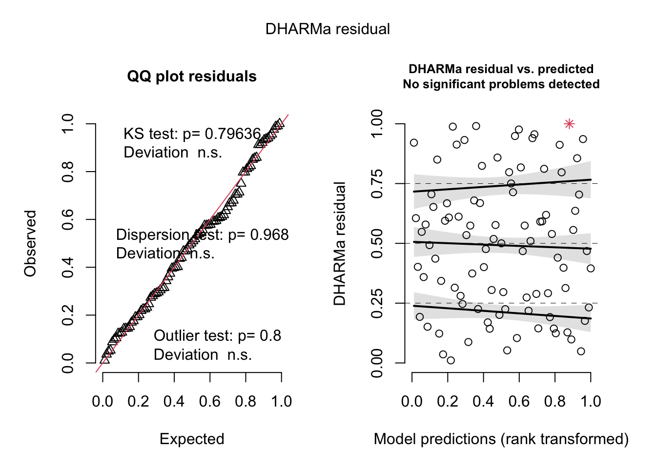
plotResiduals(res, hurricanes$NDAM)

plotResiduals(res, hurricanes$MasFem)

plotResiduals(res, hurricanes$Minpressure_Updated_2014)

No significant deviation in the general DHARMa plot, but residuals ~ NDAM looks funny, which was also pointed out by Bob O’Hara in a blog post after publication of the paper. Let’s try to correct this - scaling with ^0.2 does a great job:

correctedModel = glmmTMB(alldeaths ~ scale(MasFem) *
                             (scale(Minpressure_Updated_2014) + scale(NDAM^0.2)),
                          data = hurricanes, family = nbinom2)

res <- simulateResiduals(correctedModel, plot = T)

plotResiduals(res, hurricanes$NDAM)

summary(correctedModel)

 Family: nbinom2  ( log )
Formula:          
alldeaths ~ scale(MasFem) * (scale(Minpressure_Updated_2014) +  
    scale(NDAM^0.2))
Data: hurricanes

     AIC      BIC   logLik deviance df.resid 
   630.8    648.5   -308.4    616.8       85 


Dispersion parameter for nbinom2 family (): 1.11 

Conditional model:
                                              Estimate Std. Error z value
(Intercept)                                    2.26430    0.10912  20.751
scale(MasFem)                                  0.05156    0.10695   0.482
scale(Minpressure_Updated_2014)               -0.03162    0.18141  -0.174
scale(NDAM^0.2)                                1.28961    0.18992   6.790
scale(MasFem):scale(Minpressure_Updated_2014) -0.02410    0.20343  -0.118
scale(MasFem):scale(NDAM^0.2)                  0.16045    0.20350   0.788
                                              Pr(>|z|)    
(Intercept)                                    < 2e-16 ***
scale(MasFem)                                    0.630    
scale(Minpressure_Updated_2014)                  0.862    
scale(NDAM^0.2)                               1.12e-11 ***
scale(MasFem):scale(Minpressure_Updated_2014)    0.906    
scale(MasFem):scale(NDAM^0.2)                    0.430    
---
Signif. codes:  0 '***' 0.001 '**' 0.01 '*' 0.05 '.' 0.1 ' ' 1

car::Anova(correctedModel)

Analysis of Deviance Table (Type II Wald chisquare tests)

Response: alldeaths
                                                Chisq Df Pr(>Chisq)    
scale(MasFem)                                  0.5732  1     0.4490    
scale(Minpressure_Updated_2014)                0.1255  1     0.7232    
scale(NDAM^0.2)                               73.5010  1     <2e-16 ***
scale(MasFem):scale(Minpressure_Updated_2014)  0.0140  1     0.9057    
scale(MasFem):scale(NDAM^0.2)                  0.6216  1     0.4304    
---
Signif. codes:  0 '***' 0.001 '**' 0.01 '*' 0.05 '.' 0.1 ' ' 1

All gone, only damage is doing the effect. This wouldn’t change with re-scaling probably, as interactions are n.s.

What if we would have fit our own model? First of all, note that if hurricane names were given randomly, we wouldn’t have to worry about confounders. However, this is not the case, hurricanes were only named randomly after 1978 or so.

plot(MasFem ~ Year, data = hurricanes)

So, we could either take the earlier data out, which would remove half of our data, or we have to worry about confounding with variables that change over time. The most obvious thing would be to take time itself (Year) in the model, to correct for temporal confounding.

Do we need other variables that are not confounders? There is two reasons to add them:

they have strong effects on the response - not adding them could lead to residual problems and increase residual variance, which increases uncertainties and cost power
we want to fit interacts.

I added NDAM to the model, because we saw earlier that it has a strong effect. I think it’s not unreasonable to check for an interaction as well.

As we have several observations per year, a conservative approach would be to add a RE on year. Note that we use year both as a fixed effect (to remove temporal trends) and a random intercept, which is perfectly fine, however.

newModel = glmmTMB(alldeaths ~ scale(MasFem) * scale(NDAM^0.2) + Year + (1|Year),
                           data = hurricanes, family = nbinom2)
summary(newModel)

 Family: nbinom2  ( log )
Formula:          
alldeaths ~ scale(MasFem) * scale(NDAM^0.2) + Year + (1 | Year)
Data: hurricanes

     AIC      BIC   logLik deviance df.resid 
   630.8    648.4   -308.4    616.8       85 

Random effects:

Conditional model:
 Groups Name        Variance  Std.Dev. 
 Year   (Intercept) 2.571e-07 0.0005071
Number of obs: 92, groups:  Year, 49

Dispersion parameter for nbinom2 family (): 1.11 

Conditional model:
                               Estimate Std. Error z value Pr(>|z|)    
(Intercept)                   -2.542287  12.730846  -0.200    0.842    
scale(MasFem)                  0.073207   0.119273   0.614    0.539    
scale(NDAM^0.2)                1.309624   0.118106  11.089   <2e-16 ***
Year                           0.002426   0.006423   0.378    0.706    
scale(MasFem):scale(NDAM^0.2)  0.179874   0.117191   1.535    0.125    
---
Signif. codes:  0 '***' 0.001 '**' 0.01 '*' 0.05 '.' 0.1 ' ' 1

car::Anova(newModel) # nothing regarding MasFem

Analysis of Deviance Table (Type II Wald chisquare tests)

Response: alldeaths
                                 Chisq Df Pr(>Chisq)    
scale(MasFem)                   0.5563  1     0.4558    
scale(NDAM^0.2)               121.9237  1     <2e-16 ***
Year                            0.1426  1     0.7057    
scale(MasFem):scale(NDAM^0.2)   2.3559  1     0.1248    
---
Signif. codes:  0 '***' 0.001 '**' 0.01 '*' 0.05 '.' 0.1 ' ' 1

The results remain that there is no effect of MasFem!

C.2 Researchers Degrees of Freedom — Skin Color and Red Cards

In 2018 Silberzahn et al. published a “meta analysis” in Advances in Methods and Practices in Psychological Science, where they had provided 29 teams with the same data set to answer one research question: “[W]hether soccer players with dark skin tone are more likely than those with light skin tone to receive red cards from referees”.

Spoiler: They found that the “[a]nalytic approaches varied widely across the teams, and the estimated effect sizes ranged from 0.89 to 2.93 (Mdn = 1.31) in odds-ratio units”, highlighting that different approaches in data analysis can yield significant variation in the results.

You can find the paper “Many Analysts, One Data Set: Making Transparent How Variations in Analytic Choices Affect Results” at: https://journals.sagepub.com/doi/10.1177/2515245917747646.

The data is in

library(EcoData)
?redCards

Task: Do a re-analysis of the data as if you were the 30th team to contribute the results to the meta analysis. You can find the data in the ecodata package, dataset redCards.

Response variable: ‘redCards’ (+‘yellowReds’?).
primary predictors: ‘rater1’, ‘rater2’
Multiple variables, potentially accounting for confounding, offsetting, grouping, … are included in the data.

The rater variable contains ratings of “two independent raters blind to the research question who, based on their profile photo, categorized players on a 5-point scale ranging from (1) very light skin to (5) very dark skin. Make sure that ‘rater1’ and ‘rater2’ are rescaled to the range 0 … 1 as described in the paper (”This variable was rescaled to be bounded by 0 (very light skin) and 1 (very dark skin) prior to the final analysis, to ensure consistency of effect sizes across the teams of analysts. The raw ratings were rescaled to 0, .25, .50, .75, and 1 to create this new scale.”)

When you’re done, have a look at the other modelling teams. Do you understand the models they fit? Note that the results are displayed in terms of odd ratios. Are your results within the range of estimates from the 29 teams in Silberzahn et al. (2018)?

Solution

C.3 Scouting Ants

Look at the dataset EcoData::scoutingAnts, and find out if there are really scouting Ants in Lasius Niger.

A base model should be:

library(EcoData)
dat = scoutingAnts[scoutingAnts$first.visit == 0,]
dat$ant_group = as.factor(dat$ant_group)
dat$ant_group_main = as.factor(dat$ant_group_main)

fit <- glm(went.phero ~ ant_group_main, data = dat)
summary(fit)


Call:
glm(formula = went.phero ~ ant_group_main, data = dat)

Deviance Residuals: 
    Min       1Q   Median       3Q      Max  
-0.6986  -0.6624   0.3014   0.3014   0.3376  

Coefficients:
                                       Estimate Std. Error t value Pr(>|t|)    
(Intercept)                             0.66239    0.02139  30.974   <2e-16 ***
ant_group_mainSecondvisit_1st_to_phero  0.03626    0.02469   1.469    0.142    
---
Signif. codes:  0 '***' 0.001 '**' 0.01 '*' 0.05 '.' 0.1 ' ' 1

(Dispersion parameter for gaussian family taken to be 0.2140339)

    Null deviance: 401.35  on 1874  degrees of freedom
Residual deviance: 400.89  on 1873  degrees of freedom
AIC: 2434.5

Number of Fisher Scoring iterations: 2

Solution

For me, it made sense to change the contrasts of the possible confounders into something more easily interpretable:

Did the side in which the pheromone was stay constant or not (testing for a directional persistence of the ants)
Was the pheromone in the left or the right arm (testing for a directional preference)

dat$directionConst = ifelse(dat$Treatment %in% c("LL", "RR"), T, F)
dat$directionPhero = as.factor(ifelse(dat$Treatment %in% c("LL", "RL"), "left", "right"))

Together with the orientation of the Maze, this makes 3 possible directional confounders, and the main predictor (if the Ant went to the pheromone in the first visit).

Adding an RE on colony is logical, and then let’s run the model:

library(lme4)

Loading required package: Matrix


Attaching package: 'lme4'

The following object is masked from 'package:nlme':

    lmList

fit1<-glmer(went.phero ~ ant_group_main
             + directionConst
             + directionPhero
             + Orientation
             + (1|Colony),family="binomial", 
             data=dat)
summary(fit1)

Generalized linear mixed model fit by maximum likelihood (Laplace
  Approximation) [glmerMod]
 Family: binomial  ( logit )
Formula: went.phero ~ ant_group_main + directionConst + directionPhero +  
    Orientation + (1 | Colony)
   Data: dat

      AIC       BIC    logLik -2*log(L)  df.resid 
   2192.5    2225.7   -1090.2    2180.5      1869 

Scaled residuals: 
    Min      1Q  Median      3Q     Max 
-4.6870 -1.0451  0.4836  0.6876  1.0318 

Random effects:
 Groups Name        Variance Std.Dev.
 Colony (Intercept) 0.9284   0.9636  
Number of obs: 1875, groups:  Colony, 15

Fixed effects:
                                       Estimate Std. Error z value Pr(>|z|)    
(Intercept)                              1.9505     0.3330   5.857 4.72e-09 ***
ant_group_mainSecondvisit_1st_to_phero   0.1311     0.1248   1.050  0.29351    
directionConstTRUE                      -1.1465     0.2409  -4.760 1.94e-06 ***
directionPheroright                     -0.5680     0.1984  -2.863  0.00420 ** 
Orientationright                        -0.3493     0.1222  -2.859  0.00425 ** 
---
Signif. codes:  0 '***' 0.001 '**' 0.01 '*' 0.05 '.' 0.1 ' ' 1

Correlation of Fixed Effects:
            (Intr) a__S_1 dCTRUE drctnP
ant_g_S_1__ -0.252                     
drctnCnTRUE -0.413 -0.062              
drctnPhrrgh -0.441 -0.001  0.306       
Orinttnrght -0.182 -0.094 -0.074  0.085

Surprisingly, we find large effects of the other variables. Because of these large effects, testing for interactions with the experimental treatment as well

fit2<-glmer(went.phero ~ ant_group_main * (
             + directionConst
             + directionPhero
             + Orientation)
             + (1|Colony),family="binomial", 
             data=dat)
summary(fit2)

Generalized linear mixed model fit by maximum likelihood (Laplace
  Approximation) [glmerMod]
 Family: binomial  ( logit )
Formula: went.phero ~ ant_group_main * (+directionConst + directionPhero +  
    Orientation) + (1 | Colony)
   Data: dat

      AIC       BIC    logLik -2*log(L)  df.resid 
   2131.2    2181.0   -1056.6    2113.2      1866 

Scaled residuals: 
    Min      1Q  Median      3Q     Max 
-6.7899 -0.8936  0.4857  0.5984  1.9020 

Random effects:
 Groups Name        Variance Std.Dev.
 Colony (Intercept) 0.9497   0.9745  
Number of obs: 1875, groups:  Colony, 15

Fixed effects:
                                                           Estimate Std. Error
(Intercept)                                                  2.7384     0.3913
ant_group_mainSecondvisit_1st_to_phero                      -0.7658     0.2763
directionConstTRUE                                          -1.9420     0.3065
directionPheroright                                         -1.8133     0.3007
Orientationright                                             0.2322     0.2345
ant_group_mainSecondvisit_1st_to_phero:directionConstTRUE    1.0466     0.2638
ant_group_mainSecondvisit_1st_to_phero:directionPheroright   1.4752     0.2664
ant_group_mainSecondvisit_1st_to_phero:Orientationright     -0.8261     0.2668
                                                           z value Pr(>|z|)    
(Intercept)                                                  6.999 2.58e-12 ***
ant_group_mainSecondvisit_1st_to_phero                      -2.772  0.00557 ** 
directionConstTRUE                                          -6.337 2.34e-10 ***
directionPheroright                                         -6.030 1.64e-09 ***
Orientationright                                             0.990  0.32202    
ant_group_mainSecondvisit_1st_to_phero:directionConstTRUE    3.967 7.28e-05 ***
ant_group_mainSecondvisit_1st_to_phero:directionPheroright   5.538 3.07e-08 ***
ant_group_mainSecondvisit_1st_to_phero:Orientationright     -3.097  0.00196 ** 
---
Signif. codes:  0 '***' 0.001 '**' 0.01 '*' 0.05 '.' 0.1 ' ' 1

Correlation of Fixed Effects:
            (Intr) an__S_1__ dCTRUE drctnP Ornttn a__S_1__:C a__S_1__:P
ant_g_S_1__ -0.532                                                     
drctnCnTRUE -0.433  0.241                                              
drctnPhrrgh -0.512  0.369     0.186                                    
Orinttnrght -0.282  0.428    -0.100  0.008                             
a__S_1__:CT  0.217 -0.443    -0.592  0.043  0.015                      
an__S_1__:P  0.342 -0.528     0.007 -0.733 -0.048 -0.072               
an__S_1__:O  0.225 -0.526     0.089  0.034 -0.845 -0.021      0.046

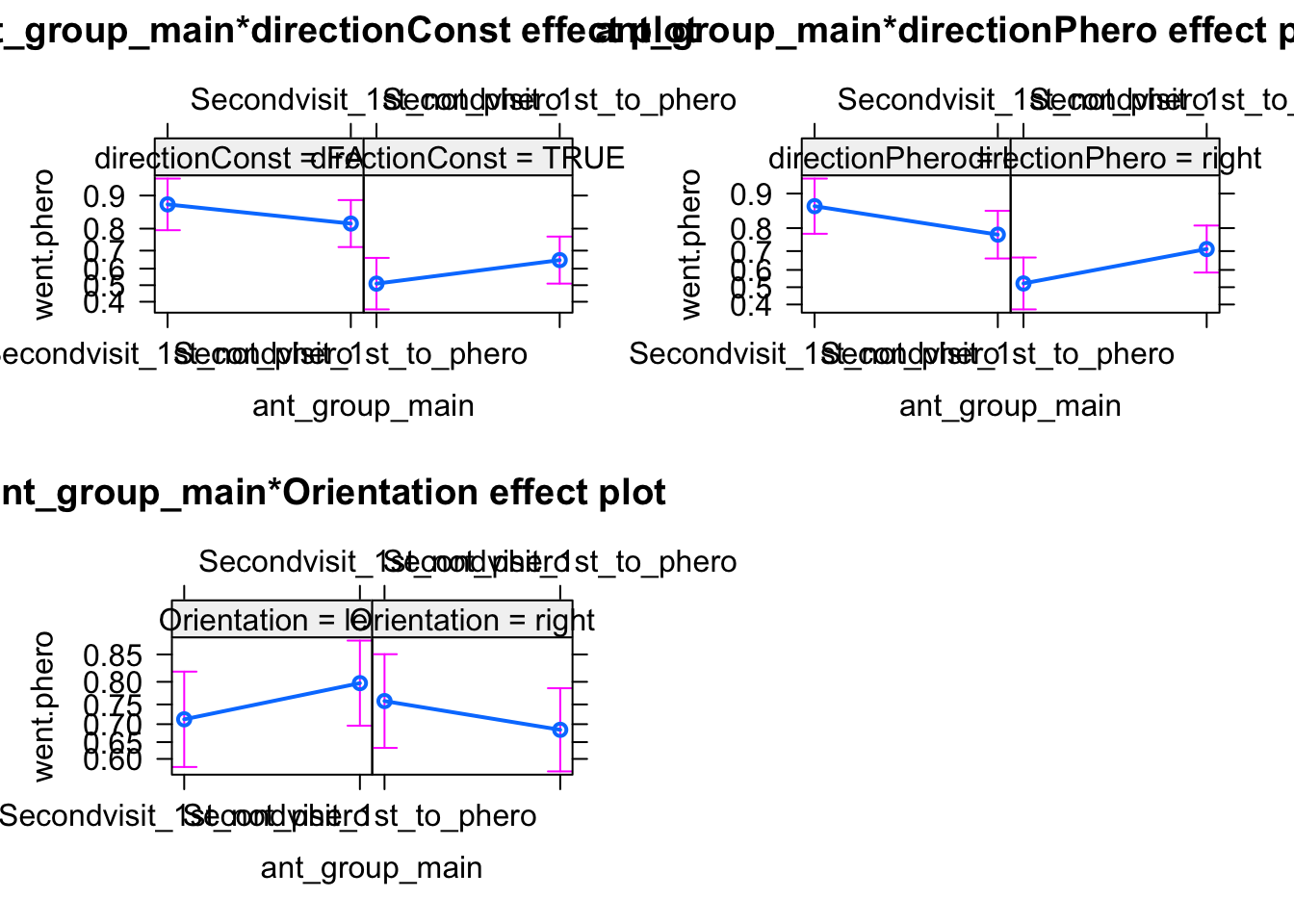
Here we find now that ther is an interaction with the main predictor, and there could be effects. We can also look at this visually.

plot(allEffects(fit2))

The results are difficult to interpret. I would think that there was some bias in the experiment, which led to an effect of the Maze direction, which then create a spill-over to the other (and in particular the main) predictors.

For our education, we can also look at the residual plots. I will use m1, because there was a misfit:

res <- simulateResiduals(m1, plot = T)

As we would significant interactions, we would probably see something if we plot residuals against predictors or their interactions, but I want to show you something else:

We will not see dispersion problems in a 0/1 binomial, but actually, this is a k/n binomial, just that the data are not prepared as such.

Either way, in DHARMa, you can aggregate residuals by a grouping variable.

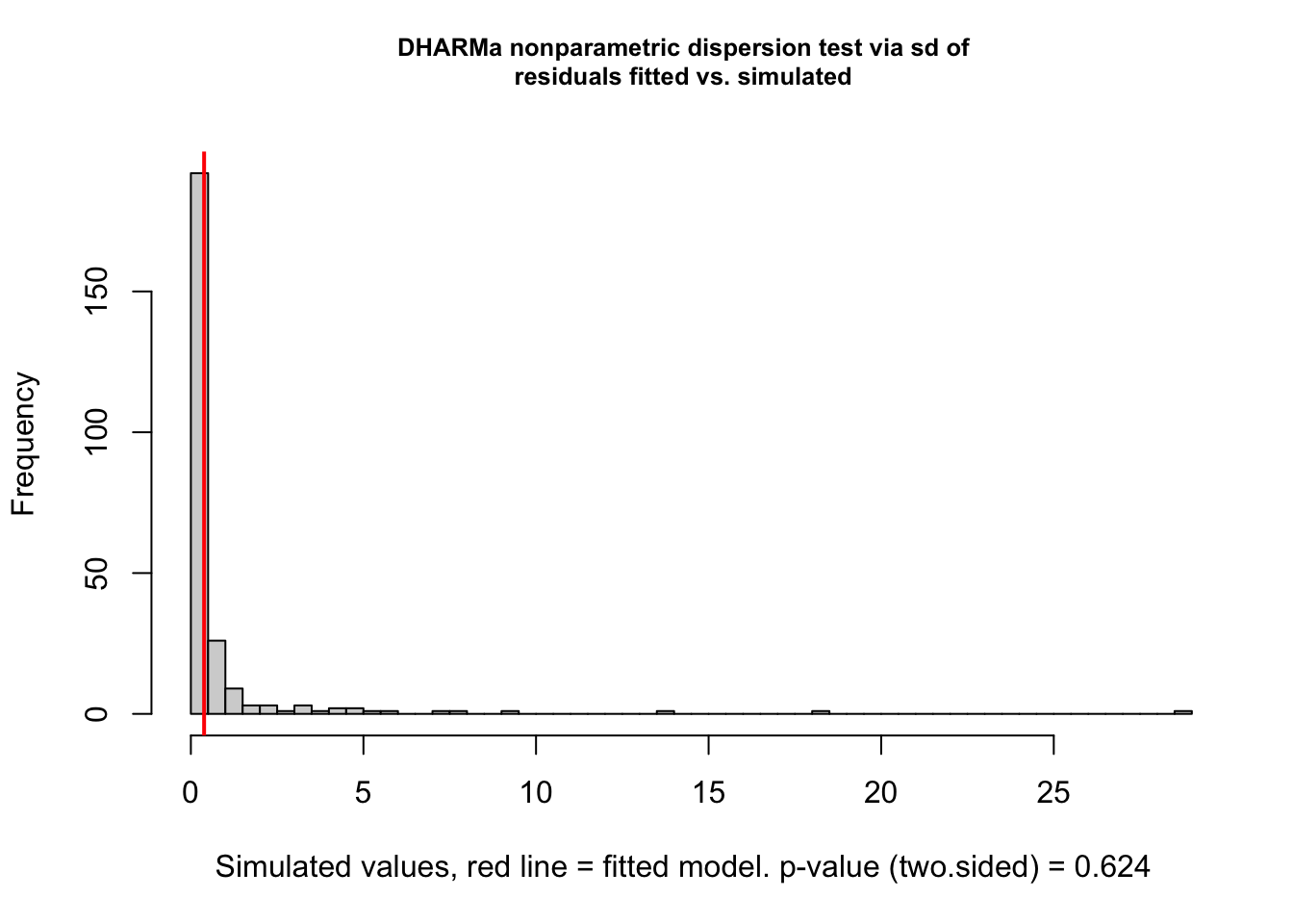
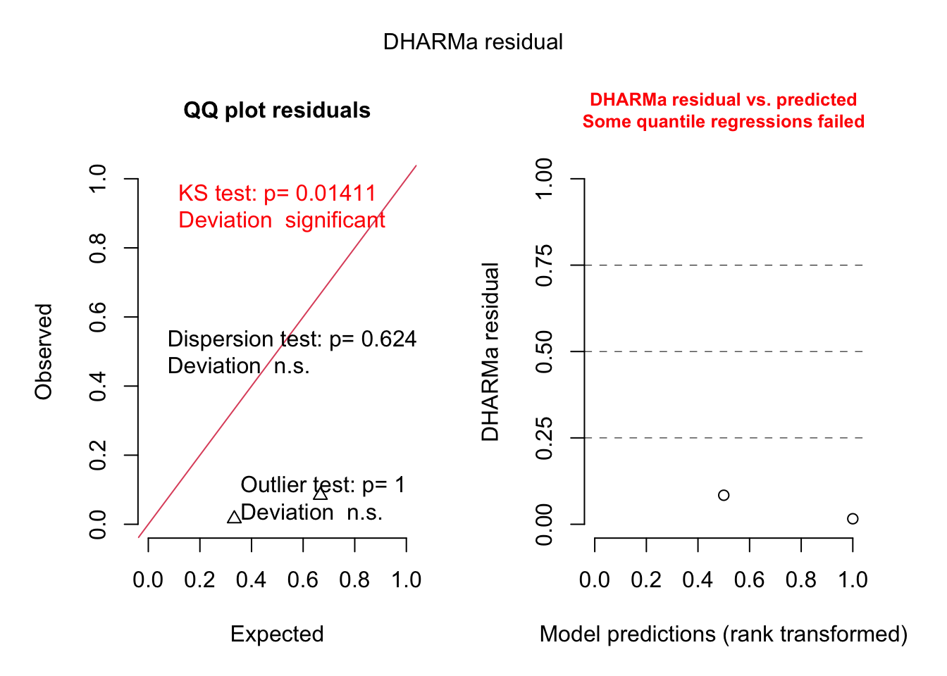
res2 <- recalculateResiduals(res, group = dat$Colony)

Now, we essentially check k/n data, and we see that there is overdispersion, which is caused by the misfit.

plot(res2)

Warning in smooth.construct.tp.smooth.spec(object, dk$data, dk$knots): basis dimension, k, increased to minimum possible


 DHARMa: qgam was unable to calculate quantile regression for quantile 0.25. Possibly to few (unique) data points / predictions. The quantile will be ommited in plots and significance calculations.

Warning in smooth.construct.tp.smooth.spec(object, dk$data, dk$knots): basis dimension, k, increased to minimum possible


 DHARMa: qgam was unable to calculate quantile regression for quantile 0.5. Possibly to few (unique) data points / predictions. The quantile will be ommited in plots and significance calculations.

Warning in smooth.construct.tp.smooth.spec(object, dk$data, dk$knots): basis dimension, k, increased to minimum possible


 DHARMa: qgam was unable to calculate quantile regression for quantile 0.75. Possibly to few (unique) data points / predictions. The quantile will be ommited in plots and significance calculations.

testDispersion(res2)


    DHARMa nonparametric dispersion test via sd of residuals fitted vs.
    simulated

data:  simulationOutput
dispersion = 0.47405, p-value = 0.624
alternative hypothesis: two.sided

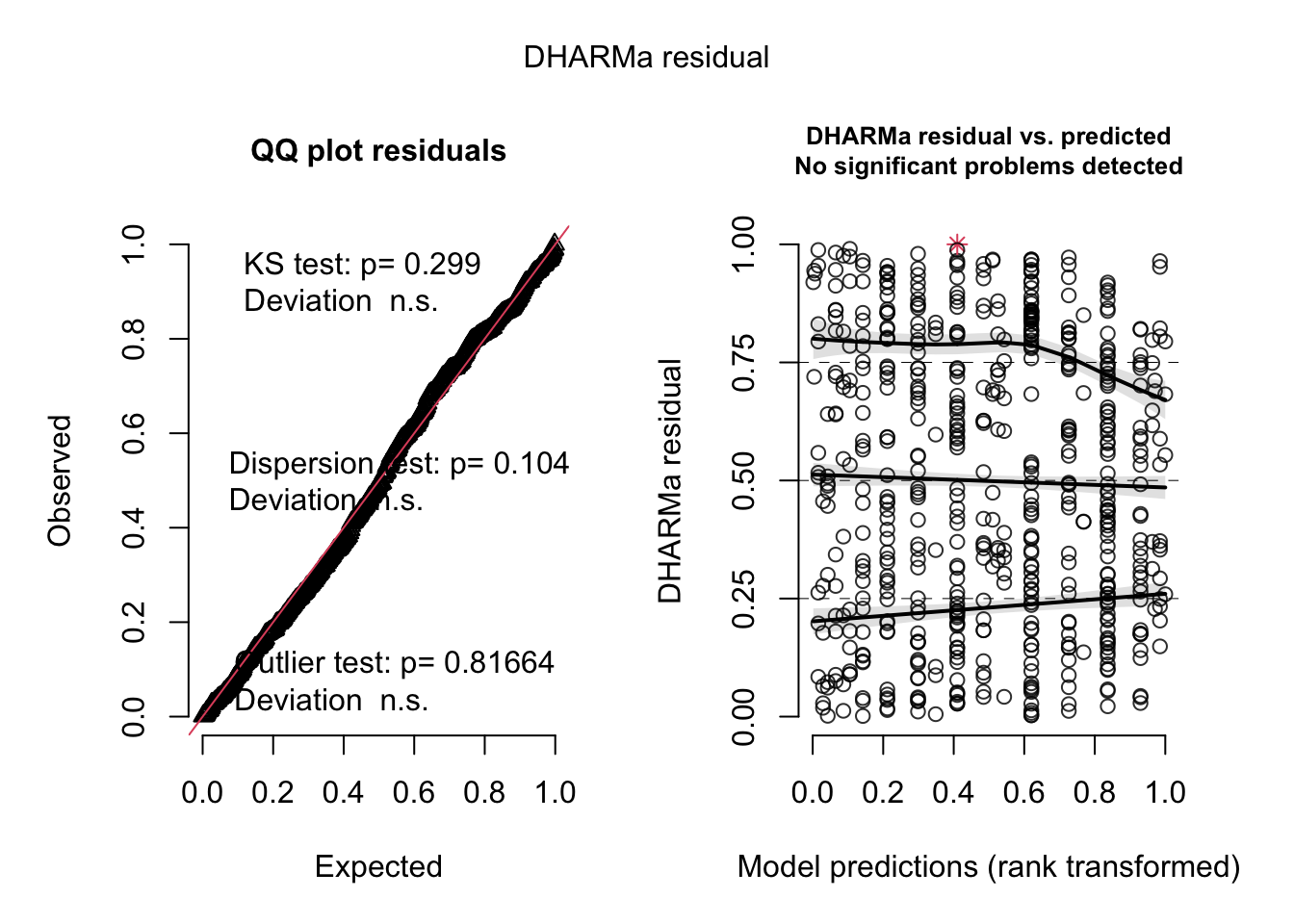
Let’s do the same for model 2, which included the interactions.

res <- simulateResiduals(m2, plot = T)

res2 <- recalculateResiduals(res, group = dat$Colony)

plot(res2)

Warning in smooth.construct.tp.smooth.spec(object, dk$data, dk$knots): basis dimension, k, increased to minimum possible


 DHARMa: qgam was unable to calculate quantile regression for quantile 0.25. Possibly to few (unique) data points / predictions. The quantile will be ommited in plots and significance calculations.

Warning in smooth.construct.tp.smooth.spec(object, dk$data, dk$knots): basis dimension, k, increased to minimum possible


 DHARMa: qgam was unable to calculate quantile regression for quantile 0.5. Possibly to few (unique) data points / predictions. The quantile will be ommited in plots and significance calculations.

Warning in smooth.construct.tp.smooth.spec(object, dk$data, dk$knots): basis dimension, k, increased to minimum possible


 DHARMa: qgam was unable to calculate quantile regression for quantile 0.75. Possibly to few (unique) data points / predictions. The quantile will be ommited in plots and significance calculations.

testDispersion(res2)


    DHARMa nonparametric dispersion test via sd of residuals fitted vs.
    simulated

data:  simulationOutput
dispersion = 0.47405, p-value = 0.624
alternative hypothesis: two.sided

Which largely removes the problem!

C.4 Owls

Look at the Owl data set in the glmmTMB package. The initial hypothesis is

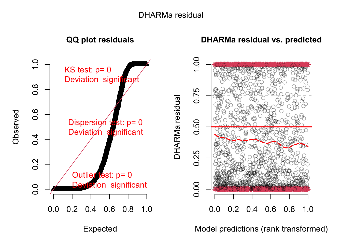
library(glmmTMB)

m1 = glm(SiblingNegotiation ~ FoodTreatment*SexParent + offset(log(BroodSize)),
         data = Owls , family = poisson)
res = simulateResiduals(m1)
plot(res)

Offset

The offset is a special command that can be used in all regression models. It means that we include an effect with effect size 1.

The offset has a special importance in models with a log link function, because with these models, we have y = exp(x …), so if you do y = exp(x + log(BroodSize) ) and use exp rules, this is y = exp(x) * exp(log(BroodSize)) = y = exp(x) * BroodSize, so this makes the response proportional to BroodSize. This trick is often used in log link GLMs to make the response proportional to Area, Sampling effort, etc.

Task: try to improve the model with everything we have discussed so far.

Solution

m1 = glmmTMB::glmmTMB(SiblingNegotiation ~ FoodTreatment * SexParent
  + (1|Nest) + offset(log(BroodSize)), data = Owls , family = nbinom1,
  dispformula = ~ FoodTreatment + SexParent,
  ziformula = ~ FoodTreatment + SexParent)
summary(m1)

 Family: nbinom1  ( log )
Formula:          
SiblingNegotiation ~ FoodTreatment * SexParent + (1 | Nest) +  
    offset(log(BroodSize))
Zero inflation:                      ~FoodTreatment + SexParent
Dispersion:                          ~FoodTreatment + SexParent
Data: Owls

     AIC      BIC   logLik deviance df.resid 
  3354.6   3402.9  -1666.3   3332.6      588 

Random effects:

Conditional model:
 Groups Name        Variance Std.Dev.
 Nest   (Intercept) 0.0876   0.296   
Number of obs: 599, groups:  Nest, 27

Conditional model:
                                    Estimate Std. Error z value Pr(>|z|)    
(Intercept)                          0.80028    0.09736   8.220  < 2e-16 ***
FoodTreatmentSatiated               -0.46893    0.16760  -2.798  0.00514 ** 
SexParentMale                       -0.09127    0.09247  -0.987  0.32363    
FoodTreatmentSatiated:SexParentMale  0.13087    0.19028   0.688  0.49158    
---
Signif. codes:  0 '***' 0.001 '**' 0.01 '*' 0.05 '.' 0.1 ' ' 1

Zero-inflation model:
                      Estimate Std. Error z value Pr(>|z|)    
(Intercept)            -1.9132     0.3269  -5.853 4.84e-09 ***
FoodTreatmentSatiated   1.0564     0.4072   2.594  0.00948 ** 
SexParentMale          -0.4688     0.3659  -1.281  0.20012    
---
Signif. codes:  0 '***' 0.001 '**' 0.01 '*' 0.05 '.' 0.1 ' ' 1

Dispersion model:
                      Estimate Std. Error z value Pr(>|z|)    
(Intercept)             1.2122     0.2214   5.475 4.37e-08 ***
FoodTreatmentSatiated   0.7978     0.2732   2.920   0.0035 ** 
SexParentMale          -0.1540     0.2399  -0.642   0.5209    
---
Signif. codes:  0 '***' 0.001 '**' 0.01 '*' 0.05 '.' 0.1 ' ' 1

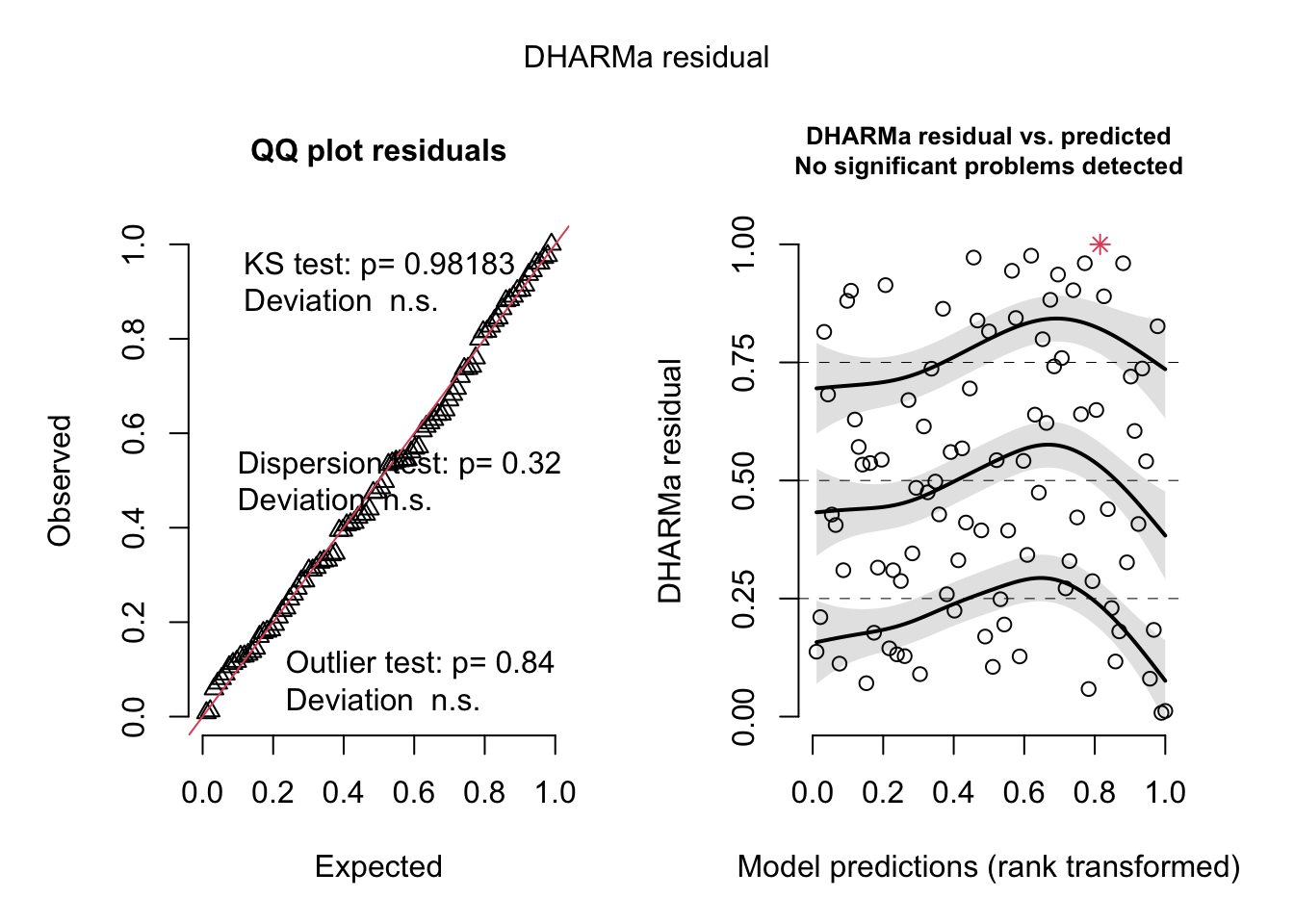
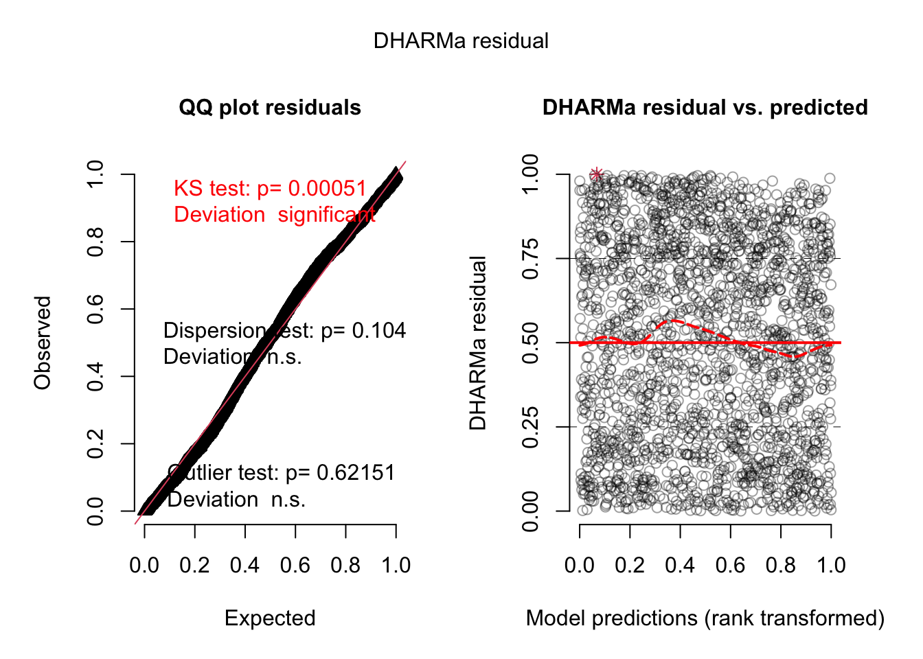
res = simulateResiduals(m1, plot = T)

testDispersion(m1)


    DHARMa nonparametric dispersion test via sd of residuals fitted vs.
    simulated

data:  simulationOutput
dispersion = 0.78311, p-value = 0.104
alternative hypothesis: two.sided

testZeroInflation(m1)


    DHARMa zero-inflation test via comparison to expected zeros with
    simulation under H0 = fitted model

data:  simulationOutput
ratioObsSim = 1.0465, p-value = 0.608
alternative hypothesis: two.sided

Solution using brms

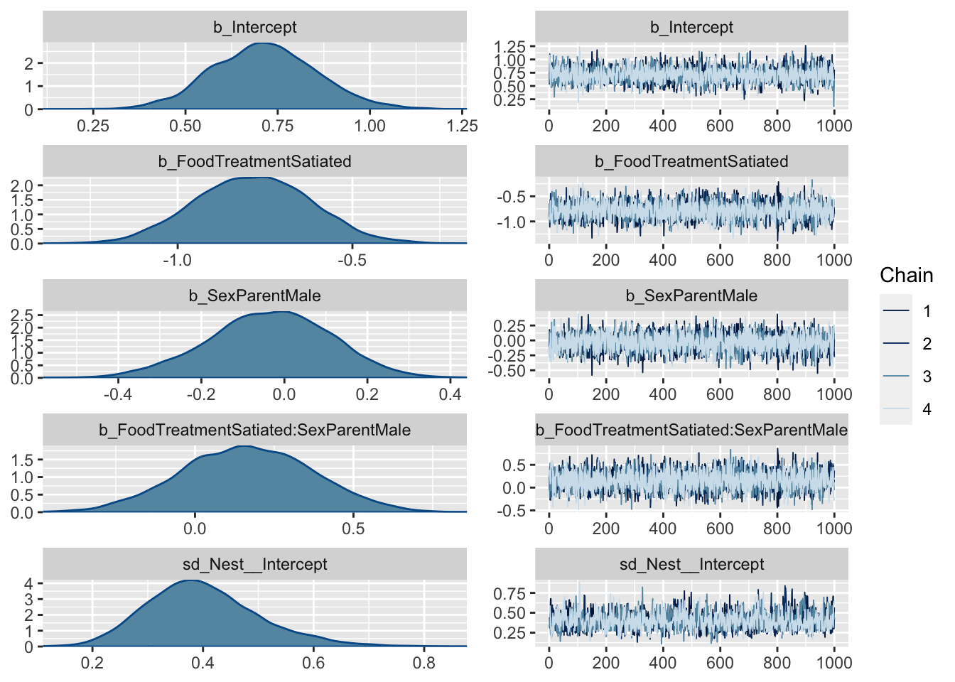
This is not adding dispersion and zero-inflation yet, just to show how such a model could be fit with brms

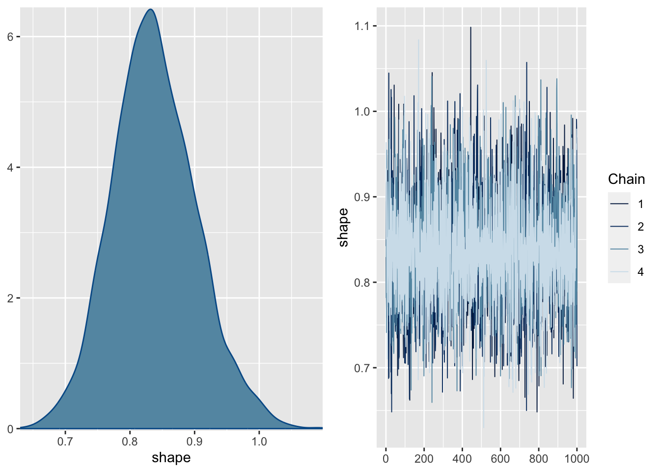
library(brms)
m2 = brms::brm(SiblingNegotiation ~ FoodTreatment * SexParent
  + (1|Nest) + offset(log(BroodSize)), 
  data = Owls , 
  family = negbinomial)


SAMPLING FOR MODEL 'anon_model' NOW (CHAIN 1).
Chain 1: 
Chain 1: Gradient evaluation took 0.000209 seconds
Chain 1: 1000 transitions using 10 leapfrog steps per transition would take 2.09 seconds.
Chain 1: Adjust your expectations accordingly!
Chain 1: 
Chain 1: 
Chain 1: Iteration:    1 / 2000 [  0%]  (Warmup)
Chain 1: Iteration:  200 / 2000 [ 10%]  (Warmup)
Chain 1: Iteration:  400 / 2000 [ 20%]  (Warmup)
Chain 1: Iteration:  600 / 2000 [ 30%]  (Warmup)
Chain 1: Iteration:  800 / 2000 [ 40%]  (Warmup)
Chain 1: Iteration: 1000 / 2000 [ 50%]  (Warmup)
Chain 1: Iteration: 1001 / 2000 [ 50%]  (Sampling)
Chain 1: Iteration: 1200 / 2000 [ 60%]  (Sampling)
Chain 1: Iteration: 1400 / 2000 [ 70%]  (Sampling)
Chain 1: Iteration: 1600 / 2000 [ 80%]  (Sampling)
Chain 1: Iteration: 1800 / 2000 [ 90%]  (Sampling)
Chain 1: Iteration: 2000 / 2000 [100%]  (Sampling)
Chain 1: 
Chain 1:  Elapsed Time: 1.328 seconds (Warm-up)
Chain 1:                1.159 seconds (Sampling)
Chain 1:                2.487 seconds (Total)
Chain 1: 

SAMPLING FOR MODEL 'anon_model' NOW (CHAIN 2).
Chain 2: 
Chain 2: Gradient evaluation took 9.1e-05 seconds
Chain 2: 1000 transitions using 10 leapfrog steps per transition would take 0.91 seconds.
Chain 2: Adjust your expectations accordingly!
Chain 2: 
Chain 2: 
Chain 2: Iteration:    1 / 2000 [  0%]  (Warmup)
Chain 2: Iteration:  200 / 2000 [ 10%]  (Warmup)
Chain 2: Iteration:  400 / 2000 [ 20%]  (Warmup)
Chain 2: Iteration:  600 / 2000 [ 30%]  (Warmup)
Chain 2: Iteration:  800 / 2000 [ 40%]  (Warmup)
Chain 2: Iteration: 1000 / 2000 [ 50%]  (Warmup)
Chain 2: Iteration: 1001 / 2000 [ 50%]  (Sampling)
Chain 2: Iteration: 1200 / 2000 [ 60%]  (Sampling)
Chain 2: Iteration: 1400 / 2000 [ 70%]  (Sampling)
Chain 2: Iteration: 1600 / 2000 [ 80%]  (Sampling)
Chain 2: Iteration: 1800 / 2000 [ 90%]  (Sampling)
Chain 2: Iteration: 2000 / 2000 [100%]  (Sampling)
Chain 2: 
Chain 2:  Elapsed Time: 1.448 seconds (Warm-up)
Chain 2:                1.292 seconds (Sampling)
Chain 2:                2.74 seconds (Total)
Chain 2: 

SAMPLING FOR MODEL 'anon_model' NOW (CHAIN 3).
Chain 3: 
Chain 3: Gradient evaluation took 9.1e-05 seconds
Chain 3: 1000 transitions using 10 leapfrog steps per transition would take 0.91 seconds.
Chain 3: Adjust your expectations accordingly!
Chain 3: 
Chain 3: 
Chain 3: Iteration:    1 / 2000 [  0%]  (Warmup)
Chain 3: Iteration:  200 / 2000 [ 10%]  (Warmup)
Chain 3: Iteration:  400 / 2000 [ 20%]  (Warmup)
Chain 3: Iteration:  600 / 2000 [ 30%]  (Warmup)
Chain 3: Iteration:  800 / 2000 [ 40%]  (Warmup)
Chain 3: Iteration: 1000 / 2000 [ 50%]  (Warmup)
Chain 3: Iteration: 1001 / 2000 [ 50%]  (Sampling)
Chain 3: Iteration: 1200 / 2000 [ 60%]  (Sampling)
Chain 3: Iteration: 1400 / 2000 [ 70%]  (Sampling)
Chain 3: Iteration: 1600 / 2000 [ 80%]  (Sampling)
Chain 3: Iteration: 1800 / 2000 [ 90%]  (Sampling)
Chain 3: Iteration: 2000 / 2000 [100%]  (Sampling)
Chain 3: 
Chain 3:  Elapsed Time: 1.303 seconds (Warm-up)
Chain 3:                1.056 seconds (Sampling)
Chain 3:                2.359 seconds (Total)
Chain 3: 

SAMPLING FOR MODEL 'anon_model' NOW (CHAIN 4).
Chain 4: 
Chain 4: Gradient evaluation took 8.8e-05 seconds
Chain 4: 1000 transitions using 10 leapfrog steps per transition would take 0.88 seconds.
Chain 4: Adjust your expectations accordingly!
Chain 4: 
Chain 4: 
Chain 4: Iteration:    1 / 2000 [  0%]  (Warmup)
Chain 4: Iteration:  200 / 2000 [ 10%]  (Warmup)
Chain 4: Iteration:  400 / 2000 [ 20%]  (Warmup)
Chain 4: Iteration:  600 / 2000 [ 30%]  (Warmup)
Chain 4: Iteration:  800 / 2000 [ 40%]  (Warmup)
Chain 4: Iteration: 1000 / 2000 [ 50%]  (Warmup)
Chain 4: Iteration: 1001 / 2000 [ 50%]  (Sampling)
Chain 4: Iteration: 1200 / 2000 [ 60%]  (Sampling)
Chain 4: Iteration: 1400 / 2000 [ 70%]  (Sampling)
Chain 4: Iteration: 1600 / 2000 [ 80%]  (Sampling)
Chain 4: Iteration: 1800 / 2000 [ 90%]  (Sampling)
Chain 4: Iteration: 2000 / 2000 [100%]  (Sampling)
Chain 4: 
Chain 4:  Elapsed Time: 1.286 seconds (Warm-up)
Chain 4:                0.931 seconds (Sampling)
Chain 4:                2.217 seconds (Total)
Chain 4:

summary(m2)

 Family: negbinomial 
  Links: mu = log; shape = identity 
Formula: SiblingNegotiation ~ FoodTreatment * SexParent + (1 | Nest) + offset(log(BroodSize)) 
   Data: Owls (Number of observations: 599) 
  Draws: 4 chains, each with iter = 2000; warmup = 1000; thin = 1;
         total post-warmup draws = 4000

Group-Level Effects: 
~Nest (Number of levels: 27) 
              Estimate Est.Error l-95% CI u-95% CI Rhat Bulk_ESS Tail_ESS
sd(Intercept)     0.39      0.10     0.21     0.61 1.00     1374     2113

Population-Level Effects: 
                                    Estimate Est.Error l-95% CI u-95% CI Rhat
Intercept                               0.72      0.14     0.45     0.99 1.00
FoodTreatmentSatiated                  -0.78      0.16    -1.09    -0.45 1.00
SexParentMale                          -0.03      0.14    -0.32     0.25 1.00
FoodTreatmentSatiated:SexParentMale     0.16      0.21    -0.25     0.56 1.00
                                    Bulk_ESS Tail_ESS
Intercept                               2668     2826
FoodTreatmentSatiated                   3341     2963
SexParentMale                           3450     3277
FoodTreatmentSatiated:SexParentMale     3242     2710

Family Specific Parameters: 
      Estimate Est.Error l-95% CI u-95% CI Rhat Bulk_ESS Tail_ESS
shape     0.84      0.07     0.72     0.98 1.00     5466     2991

Draws were sampled using sampling(NUTS). For each parameter, Bulk_ESS
and Tail_ESS are effective sample size measures, and Rhat is the potential
scale reduction factor on split chains (at convergence, Rhat = 1).

plot(m2, ask = FALSE)

C.5 Snails

library(EcoData)
library(glmmTMB)
library(lme4)
library(DHARMa)
library(tidyverse)
?EcoData::snails

Look at the Snails data set in the EcoData package, and find out which environmental and/or seasonal predictors i) explain the total abundance and ii) the infection rate of the three species.

The snails data set in the EcoData package includes observations on the distribution of freshwater snails and their infection rates ( schistosomiasis (a parasit)).

The first scientific question is that their adbundance depends on the water conditions. The second scientific question is that their infection rate depends on the water conditions and seasonsal factors

The data also contains data on other environmental (and seasonal factors). You should consider if it is useful to add them to the analysis.

Species: BP_tot, BF_tot, BT_tot

Number of infected individuals: BP_pos_tot, BF_pos_tot, BT_pos_tot

Total abundances of BP species: Bulinus_tot

Total number of infected in BP species: Bulinus_pos_tot

Tasks:

Model the summed total abundance of the three species (Bulinus_tot)
Model the infection rate of all three species (Bulinuts_pos_tot) (k/n binomial)
Optional: Model the species individually (BP_tot, BF_tot, BT_tot)
Optional: Fit a multivariate (joint) species distribution model

Solution for total Abundance of Bulinus (glmm)

Prepare+scale data:

library(lme4)
library(glmmTMB)
library(DHARMa)
data = EcoData::snails
data$sTemp_Water = scale(data$Temp_Water)
data$spH = scale(data$pH)
data$swater_speed_ms = scale(data$water_speed_ms)
data$swater_depth = scale(data$water_depth)
data$sCond = scale(data$Cond)
data$swmo_prec = scale(data$wmo_prec)
data$syear = scale(data$year)
data$sLat = scale(data$Latitude)
data$sLon = scale(data$Longitude)
data$sTemp_Air = scale(data$Temp_Air)

# Let's remove NAs beforehand:
rows = rownames(model.matrix(Bulinus_tot~sTemp_Water + spH + sLat + sLon + sCond + seas_wmo+ swmo_prec + swater_speed_ms + swater_depth +sTemp_Air+ syear + duration + locality + site_irn + coll_date, data = data))
data = data[rows, ]

Our hypothesis is that the abundance of Bulinus species depends on the water characteristics, e.g. site_type, Temp_water, pH, Cond, swmo_prec, water_speed_ms, and water_depth. We will set the length of the collection duration as an offset.

model1 = glm(Bulinus_tot~
                 offset(log(duration)) + site_type + sTemp_Water + spH +
                 sCond + swmo_prec + swater_speed_ms + swater_depth,
              data = data,  family = poisson)
summary(model1)


Call:
glm(formula = Bulinus_tot ~ offset(log(duration)) + site_type + 
    sTemp_Water + spH + sCond + swmo_prec + swater_speed_ms + 
    swater_depth, family = poisson, data = data)

Deviance Residuals: 
    Min       1Q   Median       3Q      Max  
-11.181   -5.895   -3.382    0.729   46.751  

Coefficients:
                   Estimate Std. Error z value Pr(>|z|)    
(Intercept)        0.328925   0.006417  51.258  < 2e-16 ***
site_typecanal.3  -0.161047   0.010287 -15.656  < 2e-16 ***
site_typepond     -0.837273   0.022624 -37.009  < 2e-16 ***
site_typerice.p   -1.378799   0.027252 -50.595  < 2e-16 ***
site_typeriver    -1.730850   0.032842 -52.703  < 2e-16 ***
site_typerivulet  -1.757255   0.041545 -42.298  < 2e-16 ***
site_typespillway -1.679141   0.048544 -34.590  < 2e-16 ***
sTemp_Water       -0.089050   0.004435 -20.080  < 2e-16 ***
spH                0.036653   0.004501   8.144 3.82e-16 ***
sCond              0.072787   0.004979  14.620  < 2e-16 ***
swmo_prec         -0.098717   0.006337 -15.577  < 2e-16 ***
swater_speed_ms   -0.181606   0.007695 -23.600  < 2e-16 ***
swater_depth      -0.113600   0.005998 -18.940  < 2e-16 ***
---
Signif. codes:  0 '***' 0.001 '**' 0.01 '*' 0.05 '.' 0.1 ' ' 1

(Dispersion parameter for poisson family taken to be 1)

    Null deviance: 131410  on 2071  degrees of freedom
Residual deviance: 116126  on 2059  degrees of freedom
AIC: 122311

Number of Fisher Scoring iterations: 6

As the sites are nested within localities, we will set a nested random intercept on site_irn within locality. Also potential confounders are collection date (coll_date), the season (wet or dry months, seas_wmo), year, and maybe other environmental factors such as the air temperature?.

model2 = glmer(Bulinus_tot~
                 offset(log(duration)) + site_type + sTemp_Water + spH +
                 sCond + swmo_prec + swater_speed_ms + swater_depth +
                 sTemp_Air + seas_wmo + (1|year) + (1|locality/site_irn) +  (swater_depth|coll_date),
              data = data,  family = poisson)
summary(model2)

Generalized linear mixed model fit by maximum likelihood (Laplace
  Approximation) [glmerMod]
 Family: poisson  ( log )
Formula: Bulinus_tot ~ offset(log(duration)) + site_type + sTemp_Water +  
    spH + sCond + swmo_prec + swater_speed_ms + swater_depth +  
    sTemp_Air + seas_wmo + (1 | year) + (1 | locality/site_irn) +  
    (swater_depth | coll_date)
   Data: data

      AIC       BIC    logLik -2*log(L)  df.resid 
  48873.9   48992.3  -24415.9   48831.9      2051 

Scaled residuals: 
    Min      1Q  Median      3Q     Max 
-11.997  -2.448  -0.963   1.285  41.809 

Random effects:
 Groups            Name         Variance Std.Dev. Corr
 coll_date         (Intercept)  1.8754   1.3694       
                   swater_depth 1.2493   1.1177   0.29
 site_irn:locality (Intercept)  0.7207   0.8489       
 locality          (Intercept)  0.8318   0.9120       
 year              (Intercept)  0.1613   0.4017       
Number of obs: 2072, groups:  
coll_date, 191; site_irn:locality, 89; locality, 20; year, 5

Fixed effects:
                   Estimate Std. Error z value Pr(>|z|)    
(Intercept)       -0.971159   0.363661  -2.671 0.007574 ** 
site_typecanal.3  -0.078307   0.238497  -0.328 0.742657    
site_typepond      0.291211   0.412801   0.705 0.480530    
site_typerice.p   -0.774537   0.343706  -2.253 0.024228 *  
site_typeriver    -0.532048   0.424187  -1.254 0.209741    
site_typerivulet  -0.448872   0.557398  -0.805 0.420647    
site_typespillway -0.422082   0.560277  -0.753 0.451242    
sTemp_Water       -0.055643   0.018103  -3.074 0.002114 ** 
spH               -0.029211   0.008983  -3.252 0.001147 ** 
sCond             -0.015816   0.009465  -1.671 0.094709 .  
swmo_prec         -0.212222   0.099810  -2.126 0.033481 *  
swater_speed_ms   -0.128274   0.009414 -13.626  < 2e-16 ***
swater_depth      -0.290767   0.084223  -3.452 0.000556 ***
sTemp_Air         -0.102232   0.013609  -7.512 5.82e-14 ***
seas_wmowet       -0.057522   0.205846  -0.279 0.779907    
---
Signif. codes:  0 '***' 0.001 '**' 0.01 '*' 0.05 '.' 0.1 ' ' 1


Correlation matrix not shown by default, as p = 15 > 12.
Use print(x, correlation=TRUE)  or
    vcov(x)        if you need it

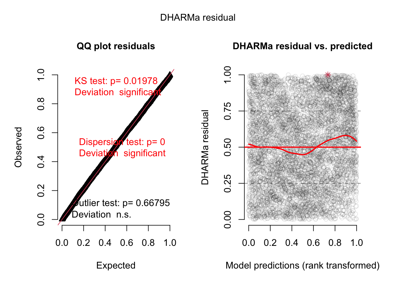
Check residuals:

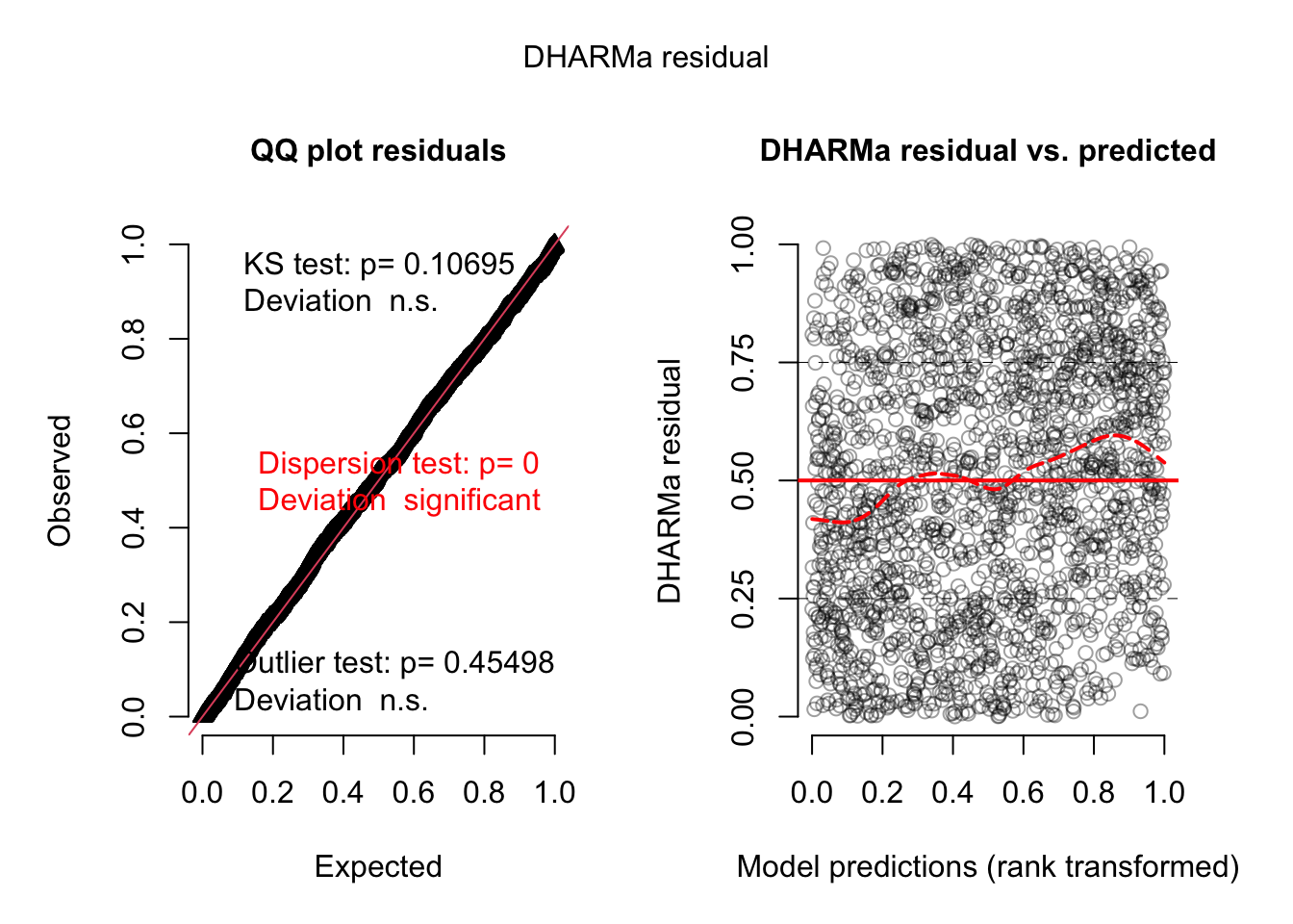
res = simulateResiduals(model2, plot = TRUE, re.form = NULL)

DHARMa:testOutliers with type = binomial may have inflated Type I error rates for integer-valued distributions. To get a more exact result, it is recommended to re-run testOutliers with type = 'bootstrap'. See ?testOutliers for details
DHARMa:testOutliers with type = binomial may have inflated Type I error rates for integer-valued distributions. To get a more exact result, it is recommended to re-run testOutliers with type = 'bootstrap'. See ?testOutliers for details

Does not look great -> dispersion problems -> switch to -> negative binomial distribution:

model3 = glmmTMB(Bulinus_tot~
                 offset(log(duration)) + site_type + sTemp_Water + spH +
                 sCond + swmo_prec + swater_speed_ms + swater_depth +
                 sTemp_Air + seas_wmo + (1|year) + (1|locality/site_irn) +  (swater_depth|coll_date),
              data = data,  family = nbinom2)
summary(model3)

 Family: nbinom2  ( log )
Formula:          
Bulinus_tot ~ offset(log(duration)) + site_type + sTemp_Water +  
    spH + sCond + swmo_prec + swater_speed_ms + swater_depth +  
    sTemp_Air + seas_wmo + (1 | year) + (1 | locality/site_irn) +  
    (swater_depth | coll_date)
Data: data

     AIC      BIC   logLik deviance df.resid 
 14137.0  14261.0  -7046.5  14093.0     2050 

Random effects:

Conditional model:
 Groups            Name         Variance Std.Dev. Corr 
 year              (Intercept)  0.32980  0.5743        
 site_irn:locality (Intercept)  0.59947  0.7743        
 locality          (Intercept)  0.54314  0.7370        
 coll_date         (Intercept)  0.66067  0.8128        
                   swater_depth 0.02441  0.1563   0.16 
Number of obs: 2072, groups:  
year, 5; site_irn:locality, 89; locality, 20; coll_date, 191

Dispersion parameter for nbinom2 family (): 0.433 

Conditional model:
                  Estimate Std. Error z value Pr(>|z|)    
(Intercept)       -0.48794    0.37886  -1.288 0.197773    
site_typecanal.3  -0.14448    0.24459  -0.591 0.554728    
site_typepond      0.09447    0.43016   0.220 0.826172    
site_typerice.p   -0.92636    0.36321  -2.550 0.010757 *  
site_typeriver    -0.82008    0.42509  -1.929 0.053709 .  
site_typerivulet  -0.98675    0.54309  -1.817 0.069231 .  
site_typespillway -0.41259    0.56965  -0.724 0.468888    
sTemp_Water       -0.10038    0.09361  -1.072 0.283532    
spH               -0.07251    0.05265  -1.377 0.168487    
sCond              0.12188    0.05953   2.047 0.040613 *  
swmo_prec         -0.10279    0.07948  -1.293 0.195908    
swater_speed_ms   -0.12390    0.03418  -3.625 0.000289 ***
swater_depth      -0.18908    0.05497  -3.440 0.000583 ***
sTemp_Air         -0.01520    0.08007  -0.190 0.849444    
seas_wmowet       -0.03143    0.17994  -0.175 0.861355    
---
Signif. codes:  0 '***' 0.001 '**' 0.01 '*' 0.05 '.' 0.1 ' ' 1

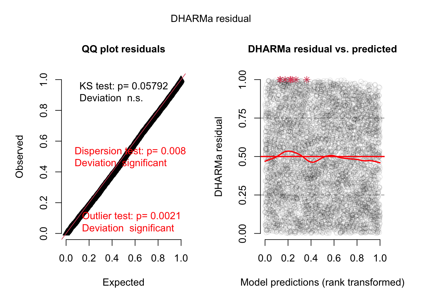
Check residuals:

res = simulateResiduals(model3, plot = TRUE)

Residuals look better but there is still a dispersion problem.

Let’s use the dispformula:

model4 = glmmTMB(Bulinus_tot~
                 offset(log(duration)) + site_type + sTemp_Water + spH +
                 sCond + swmo_prec + swater_speed_ms + swater_depth +
                 sTemp_Air + seas_wmo + (1|year) + (1|locality/site_irn) +  (swater_depth|coll_date),
                 dispformula = ~swater_speed_ms + swater_depth+sCond,
              data = data,  family = nbinom2)
summary(model4)

 Family: nbinom2  ( log )
Formula:          
Bulinus_tot ~ offset(log(duration)) + site_type + sTemp_Water +  
    spH + sCond + swmo_prec + swater_speed_ms + swater_depth +  
    sTemp_Air + seas_wmo + (1 | year) + (1 | locality/site_irn) +  
    (swater_depth | coll_date)
Dispersion:                   ~swater_speed_ms + swater_depth + sCond
Data: data

     AIC      BIC   logLik deviance df.resid 
 14138.2  14279.1  -7044.1  14088.2     2047 

Random effects:

Conditional model:
 Groups            Name         Variance Std.Dev. Corr 
 year              (Intercept)  0.32157  0.5671        
 site_irn:locality (Intercept)  0.60194  0.7758        
 locality          (Intercept)  0.53655  0.7325        
 coll_date         (Intercept)  0.65362  0.8085        
                   swater_depth 0.01958  0.1399   0.14 
Number of obs: 2072, groups:  
year, 5; site_irn:locality, 89; locality, 20; coll_date, 191

Conditional model:
                  Estimate Std. Error z value Pr(>|z|)    
(Intercept)       -0.46934    0.37644  -1.247 0.212485    
site_typecanal.3  -0.15293    0.24497  -0.624 0.532444    
site_typepond      0.05419    0.43145   0.126 0.900045    
site_typerice.p   -0.95968    0.36331  -2.641 0.008254 ** 
site_typeriver    -0.84089    0.42561  -1.976 0.048184 *  
site_typerivulet  -1.01483    0.54260  -1.870 0.061439 .  
site_typespillway -0.45053    0.57035  -0.790 0.429575    
sTemp_Water       -0.09780    0.09342  -1.047 0.295146    
spH               -0.07259    0.05246  -1.384 0.166427    
sCond              0.12399    0.06344   1.954 0.050647 .  
swmo_prec         -0.10189    0.07895  -1.290 0.196899    
swater_speed_ms   -0.16899    0.04665  -3.623 0.000292 ***
swater_depth      -0.17509    0.05627  -3.112 0.001861 ** 
sTemp_Air         -0.01550    0.08014  -0.193 0.846589    
seas_wmowet       -0.04867    0.17952  -0.271 0.786290    
---
Signif. codes:  0 '***' 0.001 '**' 0.01 '*' 0.05 '.' 0.1 ' ' 1

Dispersion model:
                 Estimate Std. Error z value Pr(>|z|)    
(Intercept)     -0.838268   0.038472 -21.789   <2e-16 ***
swater_speed_ms -0.095345   0.044883  -2.124   0.0336 *  
swater_depth    -0.003945   0.042073  -0.094   0.9253    
sCond           -0.013696   0.037138  -0.369   0.7123    
---
Signif. codes:  0 '***' 0.001 '**' 0.01 '*' 0.05 '.' 0.1 ' ' 1

Dispformula is significant. Residuals:

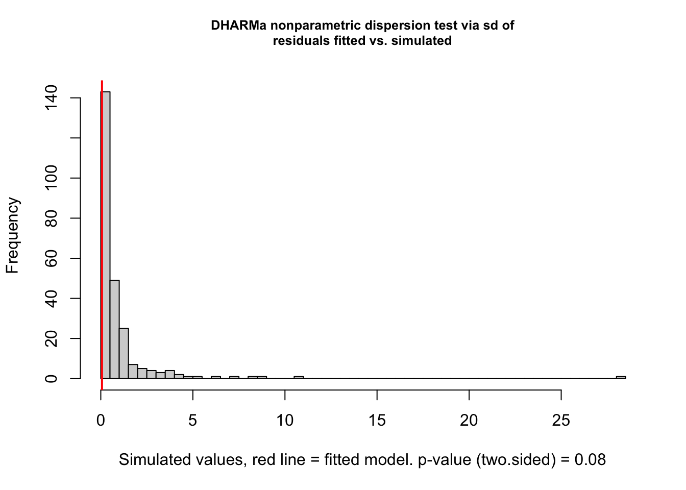
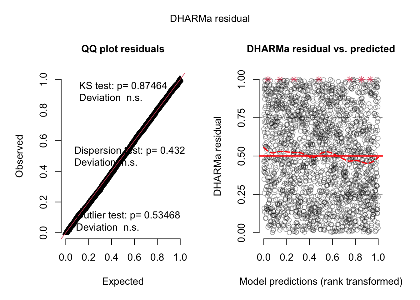
res = simulateResiduals(model4, plot = TRUE)

Dispersion tests are n.s.:

testDispersion(res)


    DHARMa nonparametric dispersion test via sd of residuals fitted vs.
    simulated

data:  simulationOutput
dispersion = 0.065593, p-value = 0.08
alternative hypothesis: two.sided

testZeroInflation(res)


    DHARMa zero-inflation test via comparison to expected zeros with
    simulation under H0 = fitted model

data:  simulationOutput
ratioObsSim = 1.052, p-value = 0.656
alternative hypothesis: two.sided

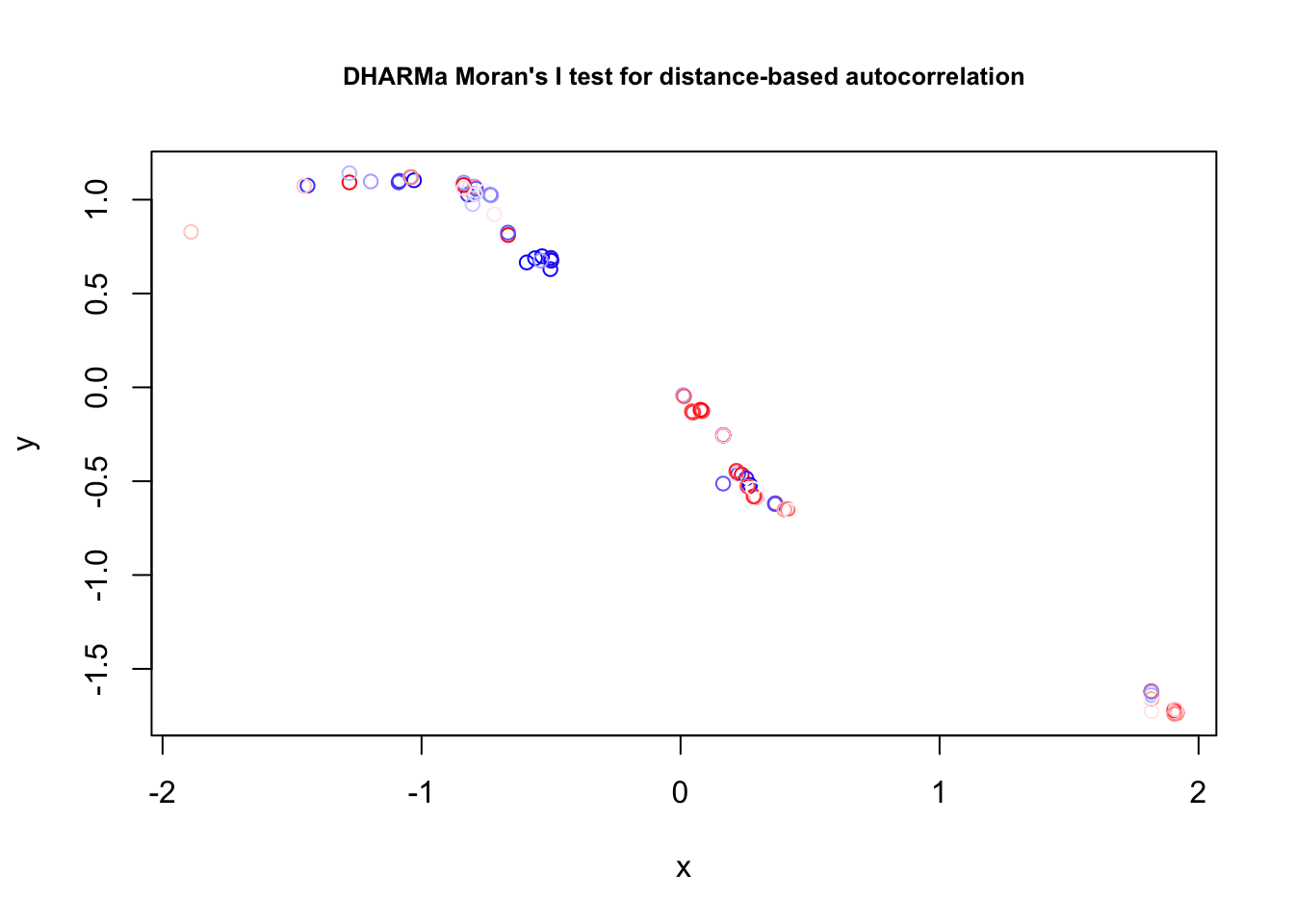
We detrended space there could be spatial autocorrelation, let’s check for it:

## Spatial
res2 = recalculateResiduals(res, group = c(data$site_irn))
groupLocations = aggregate(cbind(data$sLat, data$sLon ), list( data$site_irn), mean)
testSpatialAutocorrelation(res2, x = groupLocations$V1, y = groupLocations$V2)


    DHARMa Moran's I test for distance-based autocorrelation

data:  res2
observed = 0.295785, expected = -0.011364, sd = 0.066951, p-value =
4.482e-06
alternative hypothesis: Distance-based autocorrelation

Significant! Let’s add a spatial correlation structure:

numFac = numFactor(data$sLat, data$sLon)
group = factor(rep(1, nrow(data)))
data$fmonth = as.factor(data$month)

model5 = glmmTMB(Bulinus_tot~
                 offset(log(duration)) + site_type + sTemp_Water + spH +
                 sCond + swmo_prec + swater_speed_ms + swater_depth +
                 sTemp_Air + seas_wmo + (1|year) + (1|locality/site_irn) +  (swater_depth|coll_date) + exp(0+numFac|group),
                 dispformula = ~swater_speed_ms + swater_depth+sCond,
              data = data,  family = nbinom2)

res = simulateResiduals(model5, plot = TRUE)

DHARMa:testOutliers with type = binomial may have inflated Type I error rates for integer-valued distributions. To get a more exact result, it is recommended to re-run testOutliers with type = 'bootstrap'. See ?testOutliers for details
DHARMa:testOutliers with type = binomial may have inflated Type I error rates for integer-valued distributions. To get a more exact result, it is recommended to re-run testOutliers with type = 'bootstrap'. See ?testOutliers for details

glmmTMB does not support conditional simulations but we can create conditional simulations on our own:

pred = predict(model5, re.form = NULL, type = "response")
pred_dispersion = predict(model5, re.form = NULL, type = "disp")
simulations = sapply(1:1000, function(i) rnbinom(length(pred),size = pred_dispersion, mu =  pred))
res = createDHARMa(simulations, model.frame(model5)[,1], pred)
plot(res)

Residuals do not look perfect but I would say that we can stop here now.

Solution for prevalence of Bulinus (glmm)

Prepare+scale data:

library(lme4)
library(glmmTMB)
library(DHARMa)
data = EcoData::snails
data$sTemp_Water = scale(data$Temp_Water)
data$spH = scale(data$pH)
data$swater_speed_ms = scale(data$water_speed_ms)
data$swater_depth = scale(data$water_depth)
data$sCond = scale(data$Cond)
data$swmo_prec = scale(data$wmo_prec)
data$syear = scale(data$year)
data$sLat = scale(data$Latitude)
data$sLon = scale(data$Longitude)
data$sTemp_Air = scale(data$Temp_Air)

# Let's remove NAs beforehand:
rows = rownames(model.matrix(Bulinus_tot~sTemp_Water + spH + sLat + sLon + sCond + seas_wmo+ swmo_prec + swater_speed_ms + swater_depth +sTemp_Air+ syear + duration + locality + site_irn + coll_date, data = data))
data = data[rows, ]

Let’s start directly with all potential confounders (see previous solution):

model1 = glmmTMB(cbind(Bulinus_pos_tot, Bulinus_tot - Bulinus_pos_tot )~
                 offset(log(duration)) + site_type + sTemp_Water + spH +
                 sCond + swmo_prec + swater_speed_ms + swater_depth +
                 sTemp_Air + seas_wmo + (1|year) + (1|locality/site_irn) +  (swater_depth|coll_date),
              data = data,  family = binomial)
summary(model1)

 Family: binomial  ( logit )
Formula:          
cbind(Bulinus_pos_tot, Bulinus_tot - Bulinus_pos_tot) ~ offset(log(duration)) +  
    site_type + sTemp_Water + spH + sCond + swmo_prec + swater_speed_ms +  
    swater_depth + sTemp_Air + seas_wmo + (1 | year) + (1 | locality/site_irn) +  
    (swater_depth | coll_date)
Data: data

     AIC      BIC   logLik deviance df.resid 
  1323.3   1441.7   -640.7   1281.3     2051 

Random effects:

Conditional model:
 Groups            Name         Variance Std.Dev. Corr 
 year              (Intercept)  0.04167  0.2041        
 site_irn:locality (Intercept)  1.79468  1.3397        
 locality          (Intercept)  0.91215  0.9551        
 coll_date         (Intercept)  1.40999  1.1874        
                   swater_depth 0.46082  0.6788   0.76 
Number of obs: 2072, groups:  
year, 5; site_irn:locality, 89; locality, 20; coll_date, 191

Conditional model:
                  Estimate Std. Error z value Pr(>|z|)    
(Intercept)       -9.71202    0.52321 -18.562  < 2e-16 ***
site_typecanal.3  -0.20119    0.52740  -0.381  0.70285    
site_typepond      2.30894    0.81865   2.820  0.00480 ** 
site_typerice.p   -0.21964    0.84882  -0.259  0.79582    
site_typeriver    -0.05417    0.99933  -0.054  0.95677    
site_typerivulet   1.09537    1.05508   1.038  0.29918    
site_typespillway  0.84839    1.37766   0.616  0.53802    
sTemp_Water        0.02948    0.16178   0.182  0.85543    
spH               -0.08128    0.10741  -0.757  0.44919    
sCond             -0.32655    0.10527  -3.102  0.00192 ** 
swmo_prec         -0.59112    0.32596  -1.813  0.06976 .  
swater_speed_ms    0.17271    0.08010   2.156  0.03107 *  
swater_depth      -0.27776    0.19217  -1.445  0.14835    
sTemp_Air         -0.23545    0.14630  -1.609  0.10753    
seas_wmowet       -0.36256    0.32166  -1.127  0.25969    
---
Signif. codes:  0 '***' 0.001 '**' 0.01 '*' 0.05 '.' 0.1 ' ' 1

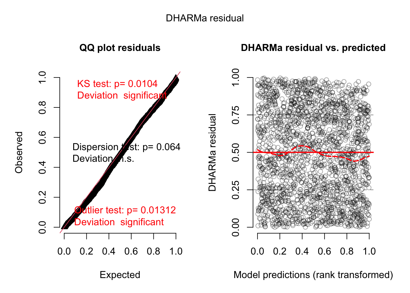
res = simulateResiduals(model1, plot=TRUE)

DHARMa:testOutliers with type = binomial may have inflated Type I error rates for integer-valued distributions. To get a more exact result, it is recommended to re-run testOutliers with type = 'bootstrap'. See ?testOutliers for details
DHARMa:testOutliers with type = binomial may have inflated Type I error rates for integer-valued distributions. To get a more exact result, it is recommended to re-run testOutliers with type = 'bootstrap'. See ?testOutliers for details

We have dispersion problems, but we cannot model the dispersion for binomial models.

Check for spatial autocorrelation:

## Spatial
res2 = recalculateResiduals(res, group = c(data$site_irn))
groupLocations = aggregate(cbind(data$sLat, data$sLon ), list( data$site_irn), mean)
testSpatialAutocorrelation(res2, x = groupLocations$V1, y = groupLocations$V2)


    DHARMa Moran's I test for distance-based autocorrelation

data:  res2
observed = 0.159982, expected = -0.011364, sd = 0.067031, p-value =
0.01058
alternative hypothesis: Distance-based autocorrelation

Significant! Let’s correct for spatial autocorrelation with a correlation structure:

numFac = numFactor(data$sLat, data$sLon)
group = factor(rep(1, nrow(data)))
data$fmonth = as.factor(data$month)
model2 = glmmTMB(cbind(Bulinus_pos_tot, Bulinus_tot - Bulinus_pos_tot )~
                 offset(log(duration)) + site_type + sTemp_Water + spH +
                 sCond + swmo_prec + swater_speed_ms + swater_depth +
                 sTemp_Air + seas_wmo + (1|year) + (1|locality/site_irn) +  (swater_depth|coll_date) + exp(0+numFac|group),
              data = data,  family = binomial)

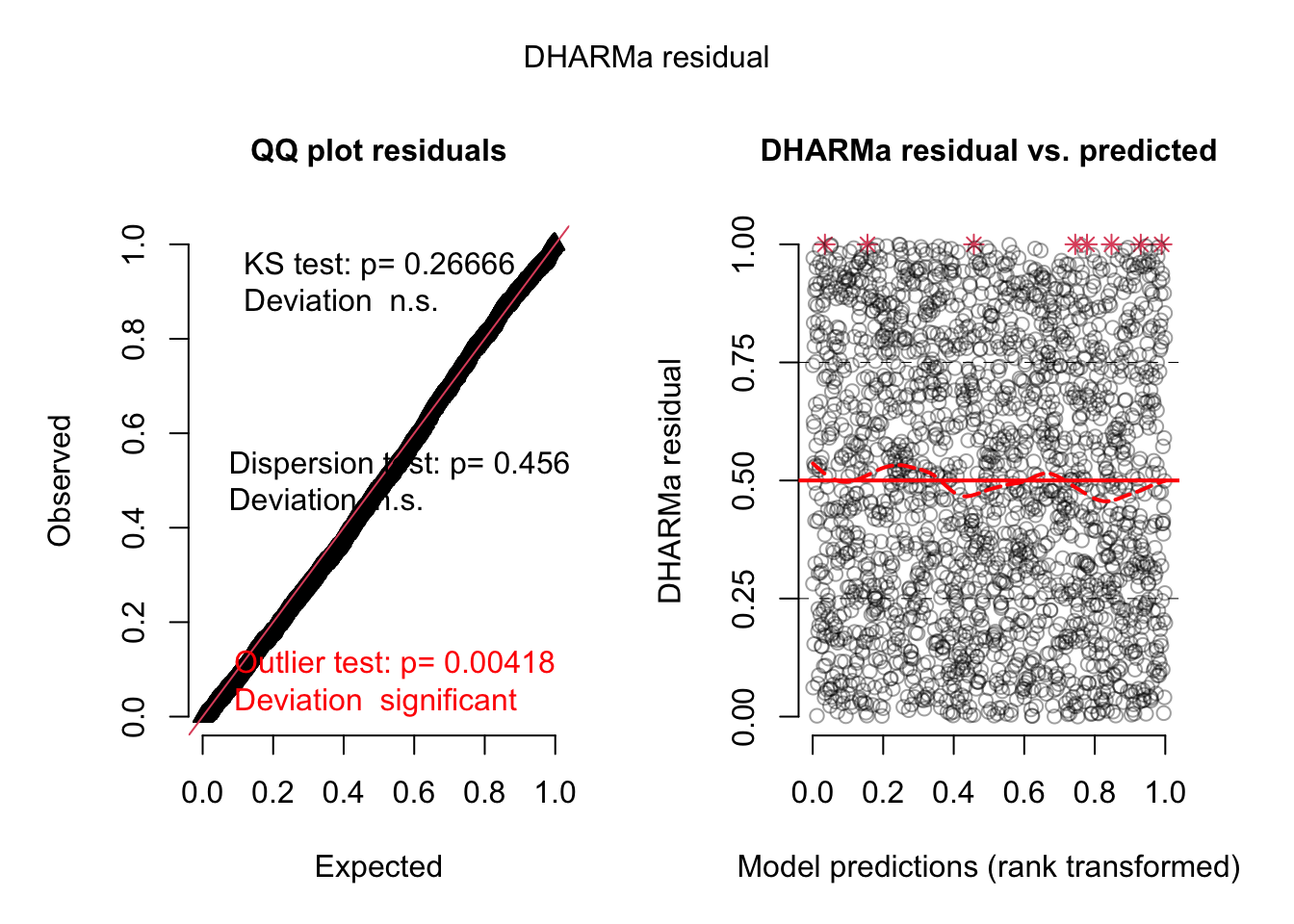
res = simulateResiduals(model2, plot = TRUE)

They look good now!

Solution of multivariate (joint) species distribution model

The species models are connected by their response to latent variable (unobserved environment). For that, we will transform our dataset with respect to species from wide (sp1, sp2, sp3) to long format (species abundances in one column and a second column telling us the group (species)). In the model then, we will separate the species and their responses by using ~0+Species + Species:(predictors).

The latent variable structure is set by the rr(…) object in the formula:

library(lme4)
library(glmmTMB)
library(DHARMa)
library(tidyverse)
data = EcoData::snails
data$sTemp_Water = scale(data$Temp_Water)
data$spH = scale(data$pH)
data$swater_speed_ms = scale(data$water_speed_ms)
data$swater_depth = scale(data$water_depth)
data$sCond = scale(data$Cond)
data$swmo_prec = scale(data$wmo_prec)
data$syear = scale(data$year)
data$sLat = scale(data$Latitude)
data$sLon = scale(data$Longitude)
data$sTemp_Air = scale(data$Temp_Air)

# Let's remove NAs beforehand:
rows = rownames(model.matrix(cbind(Bulinus_pos_tot, Bulinus_tot-Bulinus_pos_tot)~sTemp_Water + spH + sLat + sLon + sCond + seas_wmo+ swmo_prec + swater_speed_ms + swater_depth +sTemp_Air+ syear + duration + locality + site_irn + coll_date, data = data))
data = data[rows, ]


data =
  data %>% pivot_longer(cols = c("BP_tot", "BF_tot", "BT_tot"),
                      names_to = "Species",
                      values_to = "Abundance" )

numFac = numFactor(data$sLat, data$sLon)
group = factor(rep(1, nrow(data)))

numFac = numFactor(data$sLat, data$sLon)
group = factor(rep(1, nrow(data)))
data$fmonth = as.factor(data$month)
modelJoint = glmmTMB(Abundance~ 0 +
                 offset(log(duration)) + Species + Species:(site_type + 
                  sTemp_Water + spH + sCond + swmo_prec + swater_speed_ms + swater_depth +
                 sTemp_Air + seas_wmo) + (1|year) + (1|locality/site_irn) +  (swater_depth|coll_date:Species) + exp(0+numFac|group) + rr(Species + 0|locality:site_irn, d = 2),
                 dispformula = ~0+Species+Species:(swater_speed_ms + swater_depth+sCond),
              data = data,  family = nbinom2)

Warning in finalizeTMB(TMBStruc, obj, fit, h, data.tmb.old): Model convergence
problem; singular convergence (7). See vignette('troubleshooting'),
help('diagnose')

Unconditional residuals:

plot(simulateResiduals(modelJoint))

Conditional residuals:

pred = predict(modelJoint, re.form = NULL, type = "response")
pred_dispersion = predict(modelJoint, re.form = NULL, type = "disp")
simulations = sapply(1:1000, function(i) rnbinom(length(pred),size = pred_dispersion, mu =  pred))
res = createDHARMa(simulations, model.frame(modelJoint)[,1], pred)
plot(res)

C.6 Seed bank

library(EcoData)
library(glmmTMB)
library(lme4)
library(lmerTest)
library(DHARMa)
library(tidyverse)
?EcoData::seedBank

The seedBank data set in the EcoData package includes observation on seed bank presence and size in different vegetaition plots.

The scientific question is if the ability of plants to build a seed bank depends on their seed traits (see help).

The data also contains data on environmental factors and plant traits. You should consider if it is useful to add them to the analysis.

Tasks:

Fit a lm/lmm with SBDensity as response
Bonus: Add phylogenetic correlation structure
Fit a glm/glmm with SBPA as response (Bonus: add phylogenetic correlation structure)

Solution for SBDensity (lmm)

Prepare+scale data:

data = as.data.frame(EcoData::seedBank)
data$sAltitude = scale(data$Altitude)
data$sSeedMass = scale(data$SeedMass)
data$sSeedShape = scale(data$SeedShape)
data$sSeedN = scale(data$SeedN)
data$sSeedPr = scale(data$SeedPr)
data$sDormRank = scale(data$DormRank)
data$sTemp = scale(data$Temp)
data$sHum = scale(data$Humidity)
data$sNitro = scale(data$Nitrogen)
data$sGrazing = scale(data$Grazing)
data$sMGT = scale(data$MGT)
data$sJwidth = scale(data$Jwidth)
data$sEpiStein = scale(data$EpiStein)
data$sMGR = scale(data$MGR)
data$sT95 = scale(data$T95)

# Let's remove NAs beforehand:
rows = rownames(model.matrix(SBDensity~sAltitude + sSeedMass + sSeedShape + sSeedN +
                               sSeedPr + sDormRank + sTemp + sHum + sNitro + sMGT + 
                               sMGR + sEpiStein + sT95 +
                               sJwidth + sGrazing + Site + Species, data = data))
data = data[rows, ]

The response is highly skewed, so it makes sense to log-transform:

hist(data$SBDensity)

data$logSBDensity = log(data$SBDensity + 1)

Let’s fit a base model with with our hypothesis that logSBDensity ~ sSeedMass (Seed Mass) + sSeedShape + sSeedN (Number of Seeds).

We set random intercepts on species and sites because we assume that there are species and site specific variations:

model1 = lmer(logSBDensity~
                sSeedMass + sSeedShape + sSeedN + 
                (1|Site) + (1|Species),
              data = data)

summary(model1)

Linear mixed model fit by REML. t-tests use Satterthwaite's method [
lmerModLmerTest]
Formula: logSBDensity ~ sSeedMass + sSeedShape + sSeedN + (1 | Site) +  
    (1 | Species)
   Data: data

REML criterion at convergence: 7531.9

Scaled residuals: 
    Min      1Q  Median      3Q     Max 
-3.6261 -0.4945 -0.0823  0.4542  3.1525 

Random effects:
 Groups   Name        Variance Std.Dev.
 Species  (Intercept) 3.0724   1.7528  
 Site     (Intercept) 0.4705   0.6859  
 Residual             3.6790   1.9181  
Number of obs: 1729, groups:  Species, 152; Site, 17

Fixed effects:
            Estimate Std. Error       df t value Pr(>|t|)    
(Intercept)   1.5314     0.2271  42.4393   6.743 3.23e-08 ***
sSeedMass    -0.3316     0.1273 175.6509  -2.604  0.00999 ** 
sSeedShape   -0.3175     0.1546 155.2402  -2.054  0.04168 *  
sSeedN       -0.1818     0.1289 165.3141  -1.410  0.16028    
---
Signif. codes:  0 '***' 0.001 '**' 0.01 '*' 0.05 '.' 0.1 ' ' 1

Correlation of Fixed Effects:
           (Intr) sSdMss sSdShp
sSeedMass  -0.037              
sSeedShape -0.034  0.168       
sSeedN     -0.031  0.039  0.077

Environmental factors can be potential confounders, let’s add them to the model:

model2 = lmer(logSBDensity~
                sSeedMass + sSeedShape + sSeedN +
                 sAltitude + sHum + 
                (1|Site) + (1|Species),
              data = data)

summary(model2)

Linear mixed model fit by REML. t-tests use Satterthwaite's method [
lmerModLmerTest]
Formula: logSBDensity ~ sSeedMass + sSeedShape + sSeedN + sAltitude +  
    sHum + (1 | Site) + (1 | Species)
   Data: data

REML criterion at convergence: 7510.7

Scaled residuals: 
    Min      1Q  Median      3Q     Max 
-3.6468 -0.5089 -0.0720  0.4388  3.2140 

Random effects:
 Groups   Name        Variance Std.Dev.
 Species  (Intercept) 3.03405  1.7419  
 Site     (Intercept) 0.06929  0.2632  
 Residual             3.68099  1.9186  
Number of obs: 1729, groups:  Species, 152; Site, 17

Fixed effects:
             Estimate Std. Error        df t value Pr(>|t|)    
(Intercept)   1.65385    0.16664 113.38609   9.925  < 2e-16 ***
sSeedMass    -0.32886    0.12662 176.33088  -2.597   0.0102 *  
sSeedShape   -0.32165    0.15372 155.68190  -2.092   0.0380 *  
sSeedN       -0.18051    0.12816 165.92065  -1.408   0.1609    
sAltitude    -0.56452    0.10125  17.10538  -5.575 3.27e-05 ***
sHum          0.14280    0.09738  14.04198   1.466   0.1646    
---
Signif. codes:  0 '***' 0.001 '**' 0.01 '*' 0.05 '.' 0.1 ' ' 1

Correlation of Fixed Effects:
           (Intr) sSdMss sSdShp sSeedN sAlttd
sSeedMass  -0.052                            
sSeedShape -0.044  0.168                     
sSeedN     -0.042  0.039  0.077              
sAltitude  -0.058  0.007 -0.012 -0.006       
sHum       -0.004 -0.008 -0.003  0.004  0.512

sSeedShape and sSeedN are now statistically significant!

Question:

What about the germination temperatures, T50/T95?

Answer:

They could be mediators, Seed Shape -> T95 -> SBDensity, so it is up to if you want to include them or not!

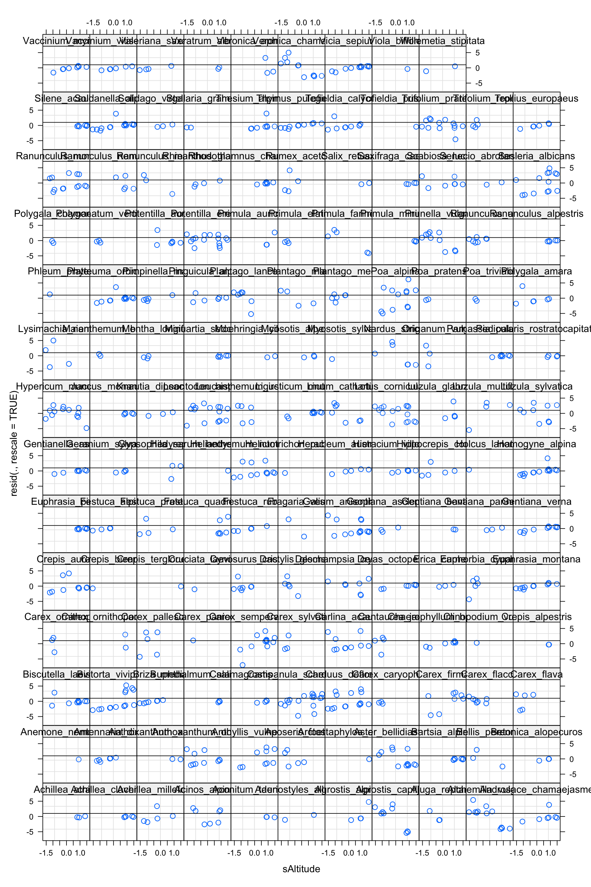
Residual checks:

Check for missing random slopes:

plot(model2, resid(., rescale=TRUE) ~ fitted(.) | Species, abline = 1)

There seems to be a pattern!

plot(model2, resid(., rescale=TRUE) ~ sAltitude | Species, abline = 1)

The pattern seems to be caused by sAltitude (check plot(model2, resid(., rescale=TRUE) ~ sSeedMass | Species, abline = 1) )

Random slope model

Let’s add a random slope on sAlitude:

model3 = lmer(logSBDensity~
                sSeedMass + sSeedShape + sSeedN +
                sAltitude + sHum + 
                (1|Site) + (sAltitude|Species),
              data = data)

summary(model3)

Linear mixed model fit by REML. t-tests use Satterthwaite's method [
lmerModLmerTest]
Formula: logSBDensity ~ sSeedMass + sSeedShape + sSeedN + sAltitude +  
    sHum + (1 | Site) + (sAltitude | Species)
   Data: data

REML criterion at convergence: 7216.1

Scaled residuals: 
     Min       1Q   Median       3Q      Max 
-2.77162 -0.39884 -0.08256  0.22365  3.06745 

Random effects:
 Groups   Name        Variance Std.Dev. Corr 
 Species  (Intercept) 2.61864  1.6182        
          sAltitude   1.31560  1.1470   -0.42
 Site     (Intercept) 0.09023  0.3004        
 Residual             2.79664  1.6723        
Number of obs: 1729, groups:  Species, 152; Site, 17

Fixed effects:
             Estimate Std. Error        df t value Pr(>|t|)    
(Intercept)   1.52436    0.16898 106.79022   9.021 8.45e-15 ***
sSeedMass    -0.29923    0.13843 181.27154  -2.162 0.031960 *  
sSeedShape   -0.25730    0.14094 145.11888  -1.826 0.069969 .  
sSeedN       -0.15018    0.11145 147.11514  -1.347 0.179918    
sAltitude    -0.59612    0.15103  54.56729  -3.947 0.000228 ***
sHum          0.09296    0.10330  13.65567   0.900 0.383740    
---
Signif. codes:  0 '***' 0.001 '**' 0.01 '*' 0.05 '.' 0.1 ' ' 1

Correlation of Fixed Effects:
           (Intr) sSdMss sSdShp sSeedN sAlttd
sSeedMass  -0.042                            
sSeedShape -0.052  0.139                     
sSeedN     -0.045  0.037  0.086              
sAltitude  -0.286  0.040 -0.021 -0.003       
sHum        0.015 -0.009 -0.009  0.004  0.367

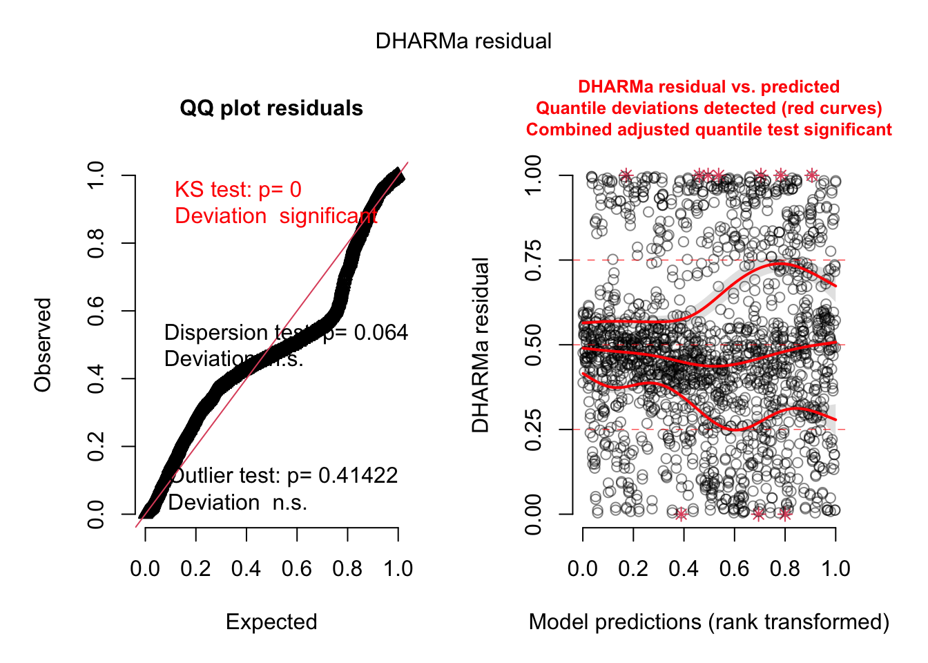
Residual checks:

plot(simulateResiduals(model3, re.form=NULL))

There seems to be dispersion problem.

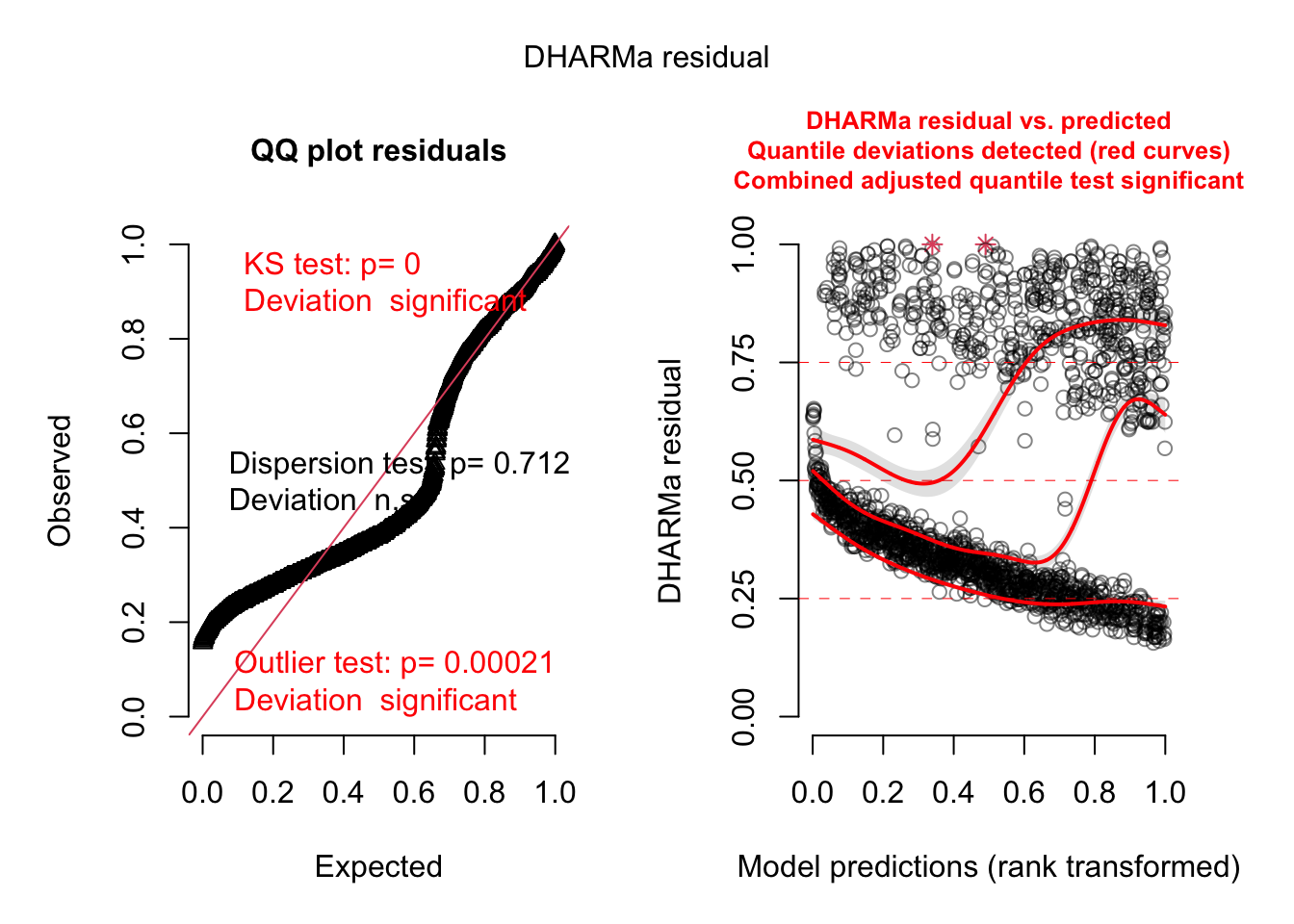
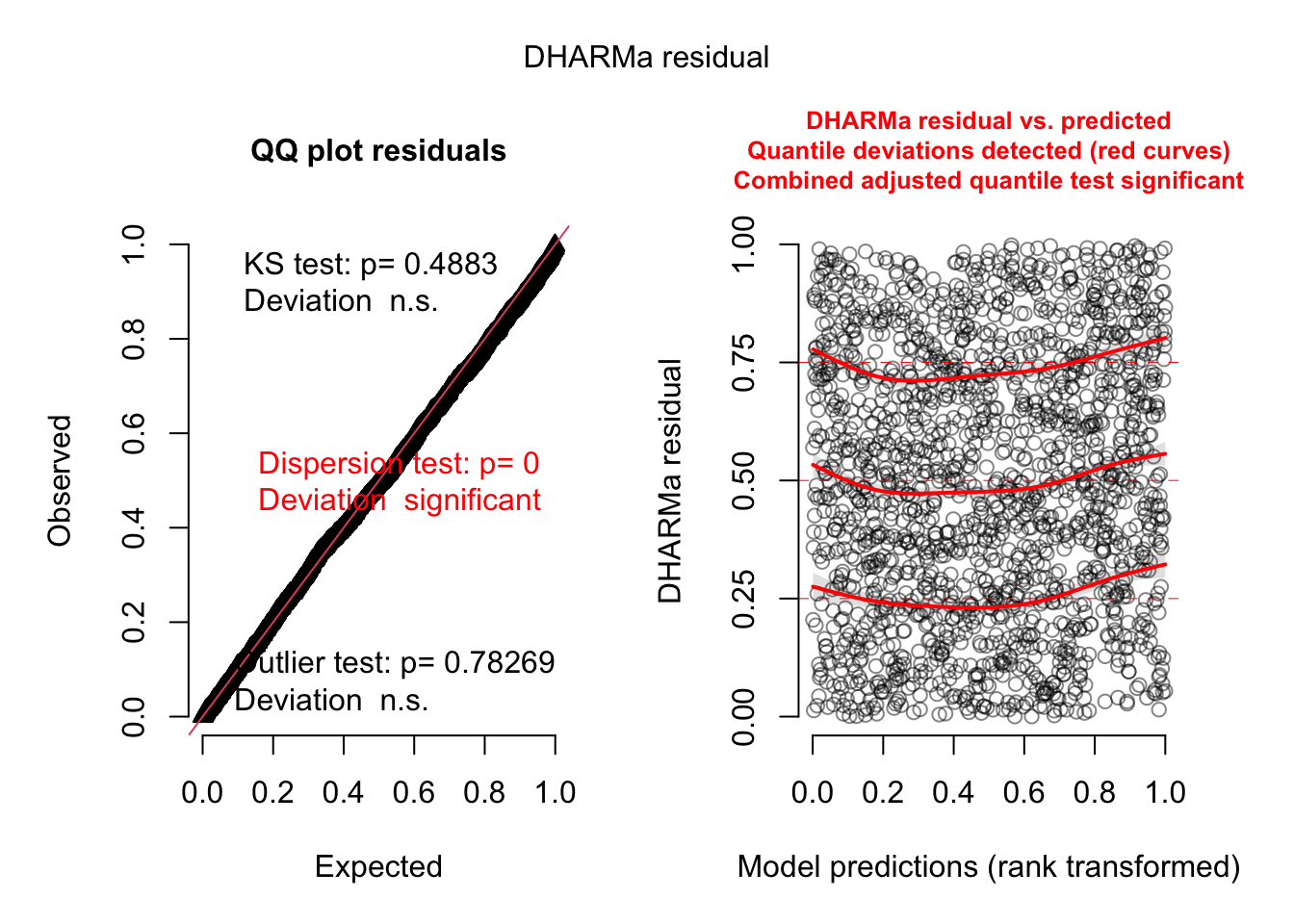
Bonus: Modeling variance with glmmTMB

model4 = glmmTMB(logSBDensity~
                sSeedMass + sSeedShape + sSeedN +
                sAltitude + sHum + 
                (1|Site) + (sAltitude|Species),
              dispformula = ~sAltitude + sHum,
              data = data)
summary(model4)

 Family: gaussian  ( identity )
Formula:          logSBDensity ~ sSeedMass + sSeedShape + sSeedN + sAltitude +  
    sHum + (1 | Site) + (sAltitude | Species)
Dispersion:                    ~sAltitude + sHum
Data: data

     AIC      BIC   logLik deviance df.resid 
  7196.3   7267.2  -3585.2   7170.3     1716 

Random effects:

Conditional model:
 Groups   Name        Variance Std.Dev. Corr  
 Site     (Intercept) 0.07148  0.2674         
 Species  (Intercept) 2.53442  1.5920         
          sAltitude   1.30195  1.1410   -0.44 
 Residual                  NA      NA         
Number of obs: 1729, groups:  Site, 17; Species, 152

Conditional model:
            Estimate Std. Error z value Pr(>|z|)    
(Intercept)  1.51412    0.16438   9.211  < 2e-16 ***
sSeedMass   -0.28914    0.13762  -2.101   0.0356 *  
sSeedShape  -0.24086    0.13832  -1.741   0.0816 .  
sSeedN      -0.14539    0.10827  -1.343   0.1793    
sAltitude   -0.59734    0.14562  -4.102 4.09e-05 ***
sHum         0.09070    0.09475   0.957   0.3384    
---
Signif. codes:  0 '***' 0.001 '**' 0.01 '*' 0.05 '.' 0.1 ' ' 1

Dispersion model:
            Estimate Std. Error z value Pr(>|z|)    
(Intercept)  0.51449    0.01856  27.713  < 2e-16 ***
sAltitude   -0.12343    0.02397  -5.148 2.63e-07 ***
sHum        -0.01575    0.02630  -0.599    0.549    
---
Signif. codes:  0 '***' 0.001 '**' 0.01 '*' 0.05 '.' 0.1 ' ' 1

Bonus: Solution for SBDensity (lmm) with phylogenetic correlation structure

Prepare phylogeny:

library(ape)


Attaching package: 'ape'

The following object is masked from 'package:dplyr':

    where

library(geiger)


Attaching package: 'geiger'

The following object is masked from 'package:brms':

    bf

species = unique(data$Species)
species_df = data.frame(Species = species)
rownames(species_df) = species
obj = name.check(plantPhylo, species_df)

# drop rest of the species
phyl.upd = drop.tip(plantPhylo, obj$tree_not_data)
summary(phyl.upd)


Phylogenetic tree: phyl.upd 

  Number of tips: 152 
  Number of nodes: 140 
  Branch lengths:
    mean: 22.21203 
    variance: 624.9334 
    distribution summary:
      Min.    1st Qu.     Median    3rd Qu.       Max. 
  0.200000   5.425002  12.800003  30.402499 123.000001 
  Root edge: 1 
  First ten tip labels: Tofieldia_pusilla 
                        Tofieldia_calyculata
                        Veratrum_album
                        Maianthemum_bifolium
                        Polygonatum_verticillatum
                        Juncus_monanthos
                        Luzula_glabrata
                        Luzula_sylvatica
                        Luzula_multiflora
                        Carex_sempervirens
  First ten node labels: N398 
                         N401
                         Tofieldiaceae
                         N573
                         N636
                         N1019
                         N1054
                         N1063
                         Juncaceae
                         Luzula

# check the names in the tree and in the data set
name.check(phyl.upd, species_df)

[1] "OK"

phyl.upd2 = multi2di(phyl.upd)

nlme:

library(nlme)
model4 = gls(logSBDensity ~
              sSeedMass + sSeedShape + sSeedN +
                 sAltitude + sHum,
             correlation = corBrownian(phy = phyl.upd2, form =~ Species),
             data = data)
summary(model4)

Generalized least squares fit by REML
  Model: logSBDensity ~ sSeedMass + sSeedShape + sSeedN + sAltitude +      sHum 
  Data: data 
        AIC     BIC   logLik
  -300576.2 -300538 150295.1

Correlation Structure: corBrownian
 Formula: ~Species 
 Parameter estimate(s):
numeric(0)

Coefficients:
                 Value Std.Error   t-value p-value
(Intercept)  1.8940733 0.7879503  2.403798  0.0163
sSeedMass   -0.3233717 0.0930947 -3.473578  0.0005
sSeedShape  -0.1898476 0.1184347 -1.602973  0.1091
sSeedN      -0.0678053 0.1180418 -0.574418  0.5658
sAltitude   -0.6393685 0.1998323 -3.199526  0.0014
sHum         0.0454568 0.1819503  0.249831  0.8027

 Correlation: 
           (Intr) sSdMss sSdShp sSeedN sAlttd
sSeedMass  -0.117                            
sSeedShape  0.041  0.048                     
sSeedN     -0.007  0.017  0.037              
sAltitude   0.167 -0.012 -0.008  0.007       
sHum        0.083  0.013  0.000 -0.007  0.621

Standardized residuals:
       Min         Q1        Med         Q3        Max 
-1.4951026 -0.8482715 -0.5644143  1.1540499  4.1762125 

Residual standard error: 2.144554 
Degrees of freedom: 1729 total; 1723 residual

glmmTMB (not perfect because lack of support of specific phylogenetic correlation structures):

dist_phylo = ape::cophenetic.phylo(phyl.upd2) # create distance matrix
correlation_matrix = vcv(phyl.upd2)[unique(data$Species), unique(data$Species)]

###
#the following code was taken from https://github.com/glmmTMB/glmmTMB/blob/master/misc/fixcorr.rmd
as.theta.vcov <- function(Sigma,corrs.only=FALSE) {
    logsd <- log(diag(Sigma))/2
    cr <- cov2cor(Sigma)
    cc <- chol(cr)
    cc <- cc %*% diag(1 / diag(cc))
    corrs <- cc[upper.tri(cc)]
    if (corrs.only) return(corrs)
    ret <- c(logsd,corrs)
    return(ret)
}
corrs = as.theta.vcov(correlation_matrix, corrs.only=TRUE)
#####

data$dummy = factor(rep(0, nrow(data)))
nsp = length(unique(data$Species))
model5 = glmmTMB(logSBDensity~
                sSeedMass + sSeedShape + sSeedN + 
                sAltitude + sHum +
                (1|Site) + (sAltitude|Species) +
                (1+Species|dummy),
              dispformula = ~sAltitude + sHum,
              map=list(theta=factor(c(rep(0, 4), rep(1,nsp),rep(NA,length(corrs))) )),
              start=list(theta=c(rep(0, 4), rep(0,nsp),corrs)),
              data = data)
summary(model5)

 Family: gaussian  ( identity )
Formula:          logSBDensity ~ sSeedMass + sSeedShape + sSeedN + sAltitude +  
    sHum + (1 | Site) + (sAltitude | Species) + (1 + Species |      dummy)
Dispersion:                    ~sAltitude + sHum
Data: data

     AIC      BIC   logLik deviance df.resid 
  7264.6   7324.6  -3621.3   7242.6     1718 

Random effects:

Conditional model:
 Groups   Name                                Variance Std.Dev. Corr          
 Site     (Intercept)                         1.022    1.011                  
 Species  (Intercept)                         1.022    1.011                  
          sAltitude                           1.022    1.011    0.01          
 dummy    (Intercept)                         2.394    1.547                  
          SpeciesAchillea_clavennae           2.394    1.547    0.00          
          SpeciesAchillea_millefolium         2.394    1.547    0.20 0.00     
          SpeciesAcinos_alpinus               2.394    1.547    0.28 0.00 0.20
          SpeciesAconitum_tauricum            2.394    1.547    0.31 0.00 0.20
          SpeciesAdenostyles_alliariae        2.394    1.547    0.00 0.93 0.00
          SpeciesAgrostis_alpina              2.394    1.547    0.20 0.00 0.34
          SpeciesAgrostis_capillaris          2.394    1.547    0.31 0.00 0.20
          SpeciesAjuga_reptans                2.394    1.547    0.31 0.00 0.20
          SpeciesAlchemilla_vulgaris          2.394    1.547    0.20 0.00 0.26
          SpeciesAndrosace_chamaejasme        2.394    1.547    0.25 0.00 0.20
          SpeciesAnemone_nemorosa             2.394    1.547    0.00 0.93 0.00
          SpeciesAntennaria_dioica            2.394    1.547    0.31 0.00 0.20
          SpeciesAnthoxanthum_alpinum         2.394    1.547    0.31 0.00 0.20
          SpeciesAnthoxanthum_odoratum        2.394    1.547    0.00 0.45 0.00
          SpeciesAnthyllis_vulneraria         2.394    1.547    0.00 0.45 0.00
          SpeciesAposeris_foetida             2.394    1.547    0.00 0.45 0.00
          SpeciesArctostaphylos_alpinus       2.394    1.547    0.00 0.45 0.00
          SpeciesAster_bellidiastrum          2.394    1.547    0.00 0.45 0.00
          SpeciesBartsia_alpina               2.394    1.547    0.00 0.45 0.00
          SpeciesBellis_perennis              2.394    1.547    0.00 0.45 0.00
          SpeciesBetonica_alopecuros          2.394    1.547    0.00 0.45 0.00
          SpeciesBiscutella_laevigata         2.394    1.547    0.00 0.45 0.00
          SpeciesBistorta_vivipara            2.394    1.547    0.31 0.00 0.20
          SpeciesBriza_media                  2.394    1.547    0.31 0.00 0.20
          SpeciesBuphthalmum_salicifolium     2.394    1.547    0.31 0.00 0.20
          SpeciesCalamagrostis_varia          2.394    1.547    0.00 0.88 0.00
          SpeciesCampanula_scheuchzeri        2.394    1.547    0.00 0.88 0.00
          SpeciesCarduus_defloratus           2.394    1.547    0.20 0.00 0.51
          SpeciesCarex_caryophyllea           2.394    1.547    0.20 0.00 0.30
          SpeciesCarex_firma                  2.394    1.547    0.55 0.00 0.20
          SpeciesCarex_flacca                 2.394    1.547    0.00 0.88 0.00
          SpeciesCarex_flava                  2.394    1.547    0.40 0.00 0.20
          SpeciesCarex_ornithopoda            2.394    1.547    0.40 0.00 0.20
          SpeciesCarex_ornithopodioides       2.394    1.547    0.20 0.00 0.26
          SpeciesCarex_pallescens             2.394    1.547    0.20 0.00 0.34
          SpeciesCarex_panicea                2.394    1.547    0.31 0.00 0.20
          SpeciesCarex_sempervirens           2.394    1.547    0.20 0.00 0.30
          SpeciesCarex_sylvatica              2.394    1.547    0.31 0.00 0.20
          SpeciesCarlina_acaulis              2.394    1.547    0.31 0.00 0.20
          SpeciesCentaurea_jacea              2.394    1.547    0.20 0.00 0.30
          SpeciesChaerophyllum_hirsutum       2.394    1.547    0.20 0.00 0.34
          SpeciesClinopodium_vulgare          2.394    1.547    0.00 0.17 0.00
          SpeciesCrepis_alpestris             2.394    1.547    0.85 0.00 0.20
          SpeciesCrepis_aurea                 2.394    1.547    0.31 0.00 0.20
          SpeciesCrepis_biennis               2.394    1.547    0.55 0.00 0.20
          SpeciesCrepis_terglouensis          2.394    1.547    0.55 0.00 0.20
          SpeciesCruciata_laevipes            2.394    1.547    0.55 0.00 0.20
          SpeciesCynosurus_cristatus          2.394    1.547    0.55 0.00 0.20
          SpeciesDactylis_glomerata           2.394    1.547    0.00 0.88 0.00
          SpeciesDeschampsia_cespitosa        2.394    1.547    0.00 0.88 0.00
          SpeciesDryas_octopetala             2.394    1.547    0.00 0.88 0.00
          SpeciesErica_carnea                 2.394    1.547    0.20 0.00 0.34
          SpeciesEuphorbia_cyparissias        2.394    1.547    0.20 0.00 0.34
          SpeciesEuphrasia_montana            2.394    1.547    0.00 0.17 0.00
          SpeciesEuphrasia_picta              2.394    1.547    0.20 0.00 0.78
          SpeciesFestuca_alpina               2.394    1.547    0.28 0.00 0.20
          SpeciesFestuca_pratensis            2.394    1.547    0.28 0.00 0.20
          SpeciesFestuca_quadriflora          2.394    1.547    0.69 0.00 0.20
          SpeciesFestuca_rubra                2.394    1.547    0.09 0.00 0.09
          SpeciesFragaria_vesca               2.394    1.547    0.09 0.00 0.09
          SpeciesGalium_anisophyllon          2.394    1.547    0.09 0.00 0.09
          SpeciesGentiana_asclepiadea         2.394    1.547    0.31 0.00 0.20
          SpeciesGentiana_bavarica            2.394    1.547    0.00 0.88 0.00
          SpeciesGentiana_pannonica           2.394    1.547    0.00 0.11 0.00
          SpeciesGentiana_verna               2.394    1.547    0.20 0.00 0.34
          SpeciesGentianella_aspera           2.394    1.547    0.20 0.00 0.34
          SpeciesGeranium_sylvaticum          2.394    1.547    0.31 0.00 0.20
          SpeciesGypsophila_repens            2.394    1.547    0.55 0.00 0.20
          SpeciesHedysarum_hedysaroides       2.394    1.547    0.55 0.00 0.20
          SpeciesHelianthemum_nummularium     2.394    1.547    0.31 0.00 0.20
          SpeciesHelictotrichon_pubescens     2.394    1.547    0.00 0.94 0.00
          SpeciesHeracleum_austriacum         2.394    1.547    0.00 0.45 0.00
          SpeciesHieracium_villosum           2.394    1.547    0.31 0.00 0.20
          SpeciesHippocrepis_comosa           2.394    1.547    0.00 0.88 0.00
          SpeciesHolcus_lanatus               2.394    1.547    0.40 0.00 0.20
          SpeciesHomogyne_alpina              2.394    1.547    0.20 0.00 0.26
          SpeciesHypericum_maculatum          2.394    1.547    0.00 0.45 0.00
          SpeciesJuncus_monanthos             2.394    1.547    0.00 0.45 0.00
          SpeciesKnautia_dipsacifolia         2.394    1.547    0.00 0.45 0.00
          SpeciesLeontodon_hispidus           2.394    1.547    0.25 0.00 0.20
          SpeciesLeucanthemum_ircutianum      2.394    1.547    0.20 0.00 0.30
          SpeciesLigusticum_mutellina         2.394    1.547    0.55 0.00 0.20
          SpeciesLinum_catharticum            2.394    1.547    0.31 0.00 0.20
          SpeciesLotus_corniculatus           2.394    1.547    0.20 0.00 0.78
          SpeciesLuzula_glabrata              2.394    1.547    0.09 0.00 0.09
          SpeciesLuzula_multiflora            2.394    1.547    0.28 0.00 0.20
          SpeciesLuzula_sylvatica             2.394    1.547    0.28 0.00 0.20
          SpeciesLysimachia_nemorum           2.394    1.547    0.09 0.00 0.09
          SpeciesMaianthemum_bifolium         2.394    1.547    0.28 0.00 0.20
          SpeciesMentha_longifolia            2.394    1.547    0.00 0.17 0.00
          SpeciesMinuartia_sedoides           2.394    1.547    0.20 0.00 0.30
          SpeciesMoehringia_ciliata           2.394    1.547    0.31 0.00 0.20
          SpeciesMyosotis_alpestris           2.394    1.547    0.31 0.00 0.20
          SpeciesMyosotis_sylvatica           2.394    1.547    0.55 0.00 0.20
          SpeciesNardus_stricta               2.394    1.547    0.00 0.88 0.00
          SpeciesOriganum_vulgare             2.394    1.547    0.40 0.00 0.20
          SpeciesParnassia_palustris          2.394    1.547    0.28 0.00 0.20
          SpeciesPedicularis_rostratocapitata 2.394    1.547    0.09 0.00 0.09
          SpeciesPhleum_pratense              2.394    1.547    0.20 0.00 0.21
          SpeciesPhyteuma_orbiculare          2.394    1.547    0.25 0.00 0.20
          SpeciesPimpinella_major             2.394    1.547    0.28 0.00 0.20
          SpeciesPinguicula_alpina            2.394    1.547    0.55 0.00 0.20
          SpeciesPlantago_lanceolata          2.394    1.547    0.20 0.00 0.34
          SpeciesPlantago_major               2.394    1.547    0.31 0.00 0.20
          SpeciesPlantago_media               2.394    1.547    0.31 0.00 0.20
          SpeciesPoa_alpina                   2.394    1.547    0.31 0.00 0.20
          SpeciesPoa_pratensis                2.394    1.547    0.00 0.88 0.00
          SpeciesPoa_trivialis                2.394    1.547    0.00 0.88 0.00
          SpeciesPolygala_amara               2.394    1.547    0.31 0.00 0.20
          SpeciesPolygala_chamaebuxus         2.394    1.547    0.31 0.00 0.20
          SpeciesPolygonatum_verticillatum    2.394    1.547    0.28 0.00 0.20
          SpeciesPotentilla_aurea             2.394    1.547    0.87 0.00 0.20
          SpeciesPotentilla_erecta            2.394    1.547    0.36 0.00 0.20
          SpeciesPrimula_auricula             2.394    1.547    0.00 0.88 0.00
          SpeciesPrimula_elatior              2.394    1.547    0.25 0.00 0.20
          SpeciesPrimula_farinosa             2.394    1.547    0.25 0.00 0.20
          SpeciesPrimula_minima               2.394    1.547    0.85 0.00 0.20
          SpeciesPrunella_vulgaris            2.394    1.547    0.31 0.00 0.20
          SpeciesRanunculus_acris             2.394    1.547    0.00 0.97 0.00
          SpeciesRanunculus_alpestris         2.394    1.547    0.65 0.00 0.20
          SpeciesRanunculus_montanus          2.394    1.547    0.28 0.00 0.20
          SpeciesRanunculus_nemorosus         2.394    1.547    0.20 0.00 0.79
          SpeciesRanunculus_repens            2.394    1.547    0.40 0.00 0.20
          SpeciesRhinanthus_glacialis         2.394    1.547    0.31 0.00 0.20
          SpeciesRhodothamnus_chamaecistus    2.394    1.547    0.31 0.00 0.20
          SpeciesRumex_acetosa                2.394    1.547    0.36 0.00 0.20
          SpeciesSalix_retusa                 2.394    1.547    0.31 0.00 0.20
          SpeciesSaxifraga_caesia             2.394    1.547    0.22 0.00 0.20
          SpeciesScabiosa_lucida              2.394    1.547    0.40 0.00 0.20
          SpeciesSenecio_abrotanifolius       2.394    1.547    0.25 0.00 0.20
          SpeciesSesleria_albicans            2.394    1.547    0.25 0.00 0.20
          SpeciesSilene_acaulis               2.394    1.547    0.20 0.00 0.30
          SpeciesSoldanella_alpina            2.394    1.547    0.09 0.00 0.09
          SpeciesSolidago_virgaurea           2.394    1.547    0.00 0.93 0.00
          SpeciesStellaria_graminea           2.394    1.547    0.00 0.45 0.00
          SpeciesThesium_alpinum              2.394    1.547    0.00 0.69 0.00
          SpeciesThymus_pulegioides           2.394    1.547    0.28 0.00 0.20
          SpeciesTofieldia_calyculata         2.394    1.547    0.00 0.88 0.00
          SpeciesTofieldia_pusilla            2.394    1.547    0.55 0.00 0.20
          SpeciesTrifolium_pratense           2.394    1.547    0.31 0.00 0.20
          SpeciesTrifolium_repens             2.394    1.547    0.00 0.88 0.00
          SpeciesTrollius_europaeus           2.394    1.547    0.63 0.00 0.20
          SpeciesVaccinium_myrtillus          2.394    1.547    0.31 0.00 0.20
          SpeciesVaccinium_vitis-idaea        2.394    1.547    0.31 0.00 0.20
          SpeciesValeriana_saxatilis          2.394    1.547    0.28 0.00 0.20
          SpeciesVeratrum_album               2.394    1.547    0.31 0.00 0.20
          SpeciesVeronica_aphylla             2.394    1.547    0.20 0.00 0.34
          SpeciesVeronica_chamaedrys          2.394    1.547    0.00 0.11 0.00
          SpeciesVicia_sepium                 2.394    1.547    0.90 0.00 0.20
          SpeciesViola_biflora                2.394    1.547    0.40 0.00 0.20
          SpeciesWillemetia_stipitata         2.394    1.547    0.09 0.00 0.09
 Residual                                        NA       NA                  
                                                                           
                                                                           
                                                                           
                                                                           
                                                                           
                                                                           
                                                                           
                                                                           
 0.28                                                                      
 0.00 0.00                                                                 
 0.20 0.20 0.00                                                            
 0.28 0.81 0.00 0.20                                                       
 0.28 0.85 0.00 0.20 0.81                                                  
 0.20 0.20 0.00 0.26 0.20 0.20                                             
 0.25 0.25 0.00 0.20 0.25 0.25 0.20                                        
 0.00 0.00 0.93 0.00 0.00 0.00 0.00 0.00                                   
 0.28 0.48 0.00 0.20 0.48 0.48 0.20 0.25 0.00                              
 0.28 0.77 0.00 0.20 0.77 0.77 0.20 0.25 0.00 0.48                         
 0.00 0.00 0.45 0.00 0.00 0.00 0.00 0.00 0.45 0.00 0.00                    
 0.00 0.00 0.45 0.00 0.00 0.00 0.00 0.00 0.45 0.00 0.00 0.91               
 0.00 0.00 0.45 0.00 0.00 0.00 0.00 0.00 0.45 0.00 0.00 0.92 0.91          
 0.00 0.00 0.45 0.00 0.00 0.00 0.00 0.00 0.45 0.00 0.00 0.92 0.91 0.92     
 0.00 0.00 0.45 0.00 0.00 0.00 0.00 0.00 0.45 0.00 0.00 0.92 0.91 0.92 0.92
 0.00 0.00 0.45 0.00 0.00 0.00 0.00 0.00 0.45 0.00 0.00 0.92 0.91 0.92 0.93
 0.00 0.00 0.45 0.00 0.00 0.00 0.00 0.00 0.45 0.00 0.00 0.92 0.91 0.92 0.92
 0.00 0.00 0.45 0.00 0.00 0.00 0.00 0.00 0.45 0.00 0.00 0.91 0.94 0.91 0.91
 0.00 0.00 0.45 0.00 0.00 0.00 0.00 0.00 0.45 0.00 0.00 0.92 0.91 0.92 0.96
 0.28 0.77 0.00 0.20 0.77 0.77 0.20 0.25 0.00 0.48 0.83 0.00 0.00 0.00 0.00
 0.28 0.77 0.00 0.20 0.77 0.77 0.20 0.25 0.00 0.48 0.90 0.00 0.00 0.00 0.00
 0.28 0.81 0.00 0.20 0.87 0.81 0.20 0.25 0.00 0.48 0.77 0.00 0.00 0.00 0.00
 0.00 0.00 0.88 0.00 0.00 0.00 0.00 0.00 0.88 0.00 0.00 0.45 0.45 0.45 0.45
 0.00 0.00 0.88 0.00 0.00 0.00 0.00 0.00 0.88 0.00 0.00 0.45 0.45 0.45 0.45
 0.20 0.20 0.00 0.34 0.20 0.20 0.26 0.20 0.00 0.20 0.20 0.00 0.00 0.00 0.00
 0.20 0.20 0.00 0.30 0.20 0.20 0.26 0.20 0.00 0.20 0.20 0.00 0.00 0.00 0.00
 0.28 0.31 0.00 0.20 0.31 0.31 0.20 0.25 0.00 0.31 0.31 0.00 0.00 0.00 0.00
 0.00 0.00 0.88 0.00 0.00 0.00 0.00 0.00 0.88 0.00 0.00 0.45 0.45 0.45 0.45
 0.28 0.31 0.00 0.20 0.31 0.31 0.20 0.25 0.00 0.31 0.31 0.00 0.00 0.00 0.00
 0.28 0.31 0.00 0.20 0.31 0.31 0.20 0.25 0.00 0.31 0.31 0.00 0.00 0.00 0.00
 0.20 0.20 0.00 0.26 0.20 0.20 0.38 0.20 0.00 0.20 0.20 0.00 0.00 0.00 0.00
 0.20 0.20 0.00 0.84 0.20 0.20 0.26 0.20 0.00 0.20 0.20 0.00 0.00 0.00 0.00
 0.28 0.83 0.00 0.20 0.81 0.83 0.20 0.25 0.00 0.48 0.77 0.00 0.00 0.00 0.00
 0.20 0.20 0.00 0.30 0.20 0.20 0.26 0.20 0.00 0.20 0.20 0.00 0.00 0.00 0.00
 0.28 0.81 0.00 0.20 0.87 0.81 0.20 0.25 0.00 0.48 0.77 0.00 0.00 0.00 0.00
 0.28 0.37 0.00 0.20 0.37 0.37 0.20 0.25 0.00 0.37 0.37 0.00 0.00 0.00 0.00
 0.20 0.20 0.00 0.30 0.20 0.20 0.26 0.20 0.00 0.20 0.20 0.00 0.00 0.00 0.00
 0.20 0.20 0.00 0.84 0.20 0.20 0.26 0.20 0.00 0.20 0.20 0.00 0.00 0.00 0.00
 0.00 0.00 0.17 0.00 0.00 0.00 0.00 0.00 0.17 0.00 0.00 0.17 0.17 0.17 0.17
 0.28 0.31 0.00 0.20 0.31 0.31 0.20 0.25 0.00 0.31 0.31 0.00 0.00 0.00 0.00
 0.28 0.37 0.00 0.20 0.37 0.37 0.20 0.25 0.00 0.37 0.37 0.00 0.00 0.00 0.00
 0.28 0.31 0.00 0.20 0.31 0.31 0.20 0.25 0.00 0.31 0.31 0.00 0.00 0.00 0.00
 0.28 0.31 0.00 0.20 0.31 0.31 0.20 0.25 0.00 0.31 0.31 0.00 0.00 0.00 0.00
 0.28 0.31 0.00 0.20 0.31 0.31 0.20 0.25 0.00 0.31 0.31 0.00 0.00 0.00 0.00
 0.28 0.31 0.00 0.20 0.31 0.31 0.20 0.25 0.00 0.31 0.31 0.00 0.00 0.00 0.00
 0.00 0.00 0.88 0.00 0.00 0.00 0.00 0.00 0.88 0.00 0.00 0.45 0.45 0.45 0.45
 0.00 0.00 0.88 0.00 0.00 0.00 0.00 0.00 0.88 0.00 0.00 0.45 0.45 0.45 0.45
 0.00 0.00 0.88 0.00 0.00 0.00 0.00 0.00 0.88 0.00 0.00 0.45 0.45 0.45 0.45
 0.20 0.20 0.00 0.43 0.20 0.20 0.26 0.20 0.00 0.20 0.20 0.00 0.00 0.00 0.00
 0.20 0.20 0.00 0.43 0.20 0.20 0.26 0.20 0.00 0.20 0.20 0.00 0.00 0.00 0.00
 0.00 0.00 0.17 0.00 0.00 0.00 0.00 0.00 0.17 0.00 0.00 0.17 0.17 0.17 0.17
 0.20 0.20 0.00 0.34 0.20 0.20 0.26 0.20 0.00 0.20 0.20 0.00 0.00 0.00 0.00
 0.72 0.28 0.00 0.20 0.28 0.28 0.20 0.25 0.00 0.28 0.28 0.00 0.00 0.00 0.00
 0.72 0.28 0.00 0.20 0.28 0.28 0.20 0.25 0.00 0.28 0.28 0.00 0.00 0.00 0.00
 0.28 0.31 0.00 0.20 0.31 0.31 0.20 0.25 0.00 0.31 0.31 0.00 0.00 0.00 0.00
 0.09 0.09 0.00 0.09 0.09 0.09 0.09 0.09 0.00 0.09 0.09 0.00 0.00 0.00 0.00
 0.09 0.09 0.00 0.09 0.09 0.09 0.09 0.09 0.00 0.09 0.09 0.00 0.00 0.00 0.00
 0.09 0.09 0.00 0.09 0.09 0.09 0.09 0.09 0.00 0.09 0.09 0.00 0.00 0.00 0.00
 0.28 0.37 0.00 0.20 0.37 0.37 0.20 0.25 0.00 0.37 0.37 0.00 0.00 0.00 0.00
 0.00 0.00 0.88 0.00 0.00 0.00 0.00 0.00 0.88 0.00 0.00 0.45 0.45 0.45 0.45
 0.00 0.00 0.11 0.00 0.00 0.00 0.00 0.00 0.11 0.00 0.00 0.11 0.11 0.11 0.11
 0.20 0.20 0.00 0.66 0.20 0.20 0.26 0.20 0.00 0.20 0.20 0.00 0.00 0.00 0.00
 0.20 0.20 0.00 0.66 0.20 0.20 0.26 0.20 0.00 0.20 0.20 0.00 0.00 0.00 0.00
 0.28 0.37 0.00 0.20 0.37 0.37 0.20 0.25 0.00 0.37 0.37 0.00 0.00 0.00 0.00
 0.28 0.31 0.00 0.20 0.31 0.31 0.20 0.25 0.00 0.31 0.31 0.00 0.00 0.00 0.00
 0.28 0.31 0.00 0.20 0.31 0.31 0.20 0.25 0.00 0.31 0.31 0.00 0.00 0.00 0.00
 0.28 0.84 0.00 0.20 0.81 0.84 0.20 0.25 0.00 0.48 0.77 0.00 0.00 0.00 0.00
 0.00 0.00 0.93 0.00 0.00 0.00 0.00 0.00 0.93 0.00 0.00 0.45 0.45 0.45 0.45
 0.00 0.00 0.45 0.00 0.00 0.00 0.00 0.00 0.45 0.00 0.00 0.92 0.91 0.92 0.92
 0.28 0.37 0.00 0.20 0.37 0.37 0.20 0.25 0.00 0.37 0.37 0.00 0.00 0.00 0.00
 0.00 0.00 0.88 0.00 0.00 0.00 0.00 0.00 0.88 0.00 0.00 0.45 0.45 0.45 0.45
 0.28 0.31 0.00 0.20 0.31 0.31 0.20 0.25 0.00 0.31 0.31 0.00 0.00 0.00 0.00
 0.20 0.20 0.00 0.26 0.20 0.20 0.27 0.20 0.00 0.20 0.20 0.00 0.00 0.00 0.00
 0.00 0.00 0.45 0.00 0.00 0.00 0.00 0.00 0.45 0.00 0.00 0.50 0.50 0.50 0.50
 0.00 0.00 0.45 0.00 0.00 0.00 0.00 0.00 0.45 0.00 0.00 0.50 0.50 0.50 0.50
 0.00 0.00 0.45 0.00 0.00 0.00 0.00 0.00 0.45 0.00 0.00 0.50 0.50 0.50 0.50
 0.25 0.25 0.00 0.20 0.25 0.25 0.20 0.43 0.00 0.25 0.25 0.00 0.00 0.00 0.00
 0.20 0.20 0.00 0.30 0.20 0.20 0.26 0.20 0.00 0.20 0.20 0.00 0.00 0.00 0.00
 0.28 0.31 0.00 0.20 0.31 0.31 0.20 0.25 0.00 0.31 0.31 0.00 0.00 0.00 0.00
 0.28 0.48 0.00 0.20 0.48 0.48 0.20 0.25 0.00 0.90 0.48 0.00 0.00 0.00 0.00
 0.20 0.20 0.00 0.34 0.20 0.20 0.26 0.20 0.00 0.20 0.20 0.00 0.00 0.00 0.00
 0.09 0.09 0.00 0.09 0.09 0.09 0.09 0.09 0.00 0.09 0.09 0.00 0.00 0.00 0.00
 0.34 0.28 0.00 0.20 0.28 0.28 0.20 0.25 0.00 0.28 0.28 0.00 0.00 0.00 0.00
 0.72 0.28 0.00 0.20 0.28 0.28 0.20 0.25 0.00 0.28 0.28 0.00 0.00 0.00 0.00
 0.09 0.09 0.00 0.09 0.09 0.09 0.09 0.09 0.00 0.09 0.09 0.00 0.00 0.00 0.00
 0.34 0.28 0.00 0.20 0.28 0.28 0.20 0.25 0.00 0.28 0.28 0.00 0.00 0.00 0.00
 0.00 0.00 0.17 0.00 0.00 0.00 0.00 0.00 0.17 0.00 0.00 0.17 0.17 0.17 0.17
 0.20 0.20 0.00 0.30 0.20 0.20 0.26 0.20 0.00 0.20 0.20 0.00 0.00 0.00 0.00
 0.28 0.85 0.00 0.20 0.81 0.86 0.20 0.25 0.00 0.48 0.77 0.00 0.00 0.00 0.00
 0.28 0.85 0.00 0.20 0.81 0.86 0.20 0.25 0.00 0.48 0.77 0.00 0.00 0.00 0.00
 0.28 0.31 0.00 0.20 0.31 0.31 0.20 0.25 0.00 0.31 0.31 0.00 0.00 0.00 0.00
 0.00 0.00 0.88 0.00 0.00 0.00 0.00 0.00 0.88 0.00 0.00 0.45 0.45 0.45 0.45
 0.28 0.31 0.00 0.20 0.31 0.31 0.20 0.25 0.00 0.31 0.31 0.00 0.00 0.00 0.00
 0.72 0.28 0.00 0.20 0.28 0.28 0.20 0.25 0.00 0.28 0.28 0.00 0.00 0.00 0.00
 0.09 0.09 0.00 0.09 0.09 0.09 0.09 0.09 0.00 0.09 0.09 0.00 0.00 0.00 0.00
 0.20 0.20 0.00 0.21 0.20 0.20 0.21 0.20 0.00 0.20 0.20 0.00 0.00 0.00 0.00
 0.25 0.25 0.00 0.20 0.25 0.25 0.20 0.43 0.00 0.25 0.25 0.00 0.00 0.00 0.00
 0.34 0.28 0.00 0.20 0.28 0.28 0.20 0.25 0.00 0.28 0.28 0.00 0.00 0.00 0.00
 0.28 0.31 0.00 0.20 0.31 0.31 0.20 0.25 0.00 0.31 0.31 0.00 0.00 0.00 0.00
 0.20 0.20 0.00 0.66 0.20 0.20 0.26 0.20 0.00 0.20 0.20 0.00 0.00 0.00 0.00
 0.28 0.85 0.00 0.20 0.81 0.86 0.20 0.25 0.00 0.48 0.77 0.00 0.00 0.00 0.00
 0.28 0.83 0.00 0.20 0.81 0.83 0.20 0.25 0.00 0.48 0.77 0.00 0.00 0.00 0.00
 0.28 0.85 0.00 0.20 0.81 0.95 0.20 0.25 0.00 0.48 0.77 0.00 0.00 0.00 0.00
 0.00 0.00 0.88 0.00 0.00 0.00 0.00 0.00 0.88 0.00 0.00 0.45 0.45 0.45 0.45
 0.00 0.00 0.88 0.00 0.00 0.00 0.00 0.00 0.88 0.00 0.00 0.45 0.45 0.45 0.45
 0.28 0.37 0.00 0.20 0.37 0.37 0.20 0.25 0.00 0.37 0.37 0.00 0.00 0.00 0.00
 0.28 0.85 0.00 0.20 0.81 0.86 0.20 0.25 0.00 0.48 0.77 0.00 0.00 0.00 0.00
 0.68 0.28 0.00 0.20 0.28 0.28 0.20 0.25 0.00 0.28 0.28 0.00 0.00 0.00 0.00
 0.28 0.31 0.00 0.20 0.31 0.31 0.20 0.25 0.00 0.31 0.31 0.00 0.00 0.00 0.00
 0.28 0.31 0.00 0.20 0.31 0.31 0.20 0.25 0.00 0.31 0.31 0.00 0.00 0.00 0.00
 0.00 0.00 0.88 0.00 0.00 0.00 0.00 0.00 0.88 0.00 0.00 0.45 0.45 0.45 0.45
 0.25 0.25 0.00 0.20 0.25 0.25 0.20 0.77 0.00 0.25 0.25 0.00 0.00 0.00 0.00
 0.25 0.25 0.00 0.20 0.25 0.25 0.20 0.43 0.00 0.25 0.25 0.00 0.00 0.00 0.00
 0.28 0.31 0.00 0.20 0.31 0.31 0.20 0.25 0.00 0.31 0.31 0.00 0.00 0.00 0.00
 0.28 0.81 0.00 0.20 0.87 0.81 0.20 0.25 0.00 0.48 0.77 0.00 0.00 0.00 0.00
 0.00 0.00 0.93 0.00 0.00 0.00 0.00 0.00 0.93 0.00 0.00 0.45 0.45 0.45 0.45
 0.28 0.31 0.00 0.20 0.31 0.31 0.20 0.25 0.00 0.31 0.31 0.00 0.00 0.00 0.00
 0.34 0.28 0.00 0.20 0.28 0.28 0.20 0.25 0.00 0.28 0.28 0.00 0.00 0.00 0.00
 0.20 0.20 0.00 0.34 0.20 0.20 0.26 0.20 0.00 0.20 0.20 0.00 0.00 0.00 0.00
 0.28 0.31 0.00 0.20 0.31 0.31 0.20 0.25 0.00 0.31 0.31 0.00 0.00 0.00 0.00
 0.28 0.81 0.00 0.20 0.86 0.81 0.20 0.25 0.00 0.48 0.77 0.00 0.00 0.00 0.00
 0.28 0.37 0.00 0.20 0.37 0.37 0.20 0.25 0.00 0.37 0.37 0.00 0.00 0.00 0.00
 0.28 0.31 0.00 0.20 0.31 0.31 0.20 0.25 0.00 0.31 0.31 0.00 0.00 0.00 0.00
 0.28 0.85 0.00 0.20 0.81 0.91 0.20 0.25 0.00 0.48 0.77 0.00 0.00 0.00 0.00
 0.22 0.22 0.00 0.20 0.22 0.22 0.20 0.22 0.00 0.22 0.22 0.00 0.00 0.00 0.00
 0.28 0.31 0.00 0.20 0.31 0.31 0.20 0.25 0.00 0.31 0.31 0.00 0.00 0.00 0.00
 0.25 0.25 0.00 0.20 0.25 0.25 0.20 0.43 0.00 0.25 0.25 0.00 0.00 0.00 0.00
 0.25 0.25 0.00 0.20 0.25 0.25 0.20 0.43 0.00 0.25 0.25 0.00 0.00 0.00 0.00
 0.20 0.20 0.00 0.30 0.20 0.20 0.26 0.20 0.00 0.20 0.20 0.00 0.00 0.00 0.00
 0.09 0.09 0.00 0.09 0.09 0.09 0.09 0.09 0.00 0.09 0.09 0.00 0.00 0.00 0.00
 0.00 0.00 0.98 0.00 0.00 0.00 0.00 0.00 0.93 0.00 0.00 0.45 0.45 0.45 0.45
 0.00 0.00 0.45 0.00 0.00 0.00 0.00 0.00 0.45 0.00 0.00 0.50 0.50 0.50 0.50
 0.00 0.00 0.69 0.00 0.00 0.00 0.00 0.00 0.69 0.00 0.00 0.45 0.45 0.45 0.45
 0.72 0.28 0.00 0.20 0.28 0.28 0.20 0.25 0.00 0.28 0.28 0.00 0.00 0.00 0.00
 0.00 0.00 0.88 0.00 0.00 0.00 0.00 0.00 0.88 0.00 0.00 0.45 0.45 0.45 0.45
 0.28 0.31 0.00 0.20 0.31 0.31 0.20 0.25 0.00 0.31 0.31 0.00 0.00 0.00 0.00
 0.28 0.81 0.00 0.20 0.87 0.81 0.20 0.25 0.00 0.48 0.77 0.00 0.00 0.00 0.00
 0.00 0.00 0.88 0.00 0.00 0.00 0.00 0.00 0.88 0.00 0.00 0.45 0.45 0.45 0.45
 0.28 0.31 0.00 0.20 0.31 0.31 0.20 0.25 0.00 0.31 0.31 0.00 0.00 0.00 0.00
 0.28 0.83 0.00 0.20 0.81 0.83 0.20 0.25 0.00 0.48 0.77 0.00 0.00 0.00 0.00
 0.28 0.81 0.00 0.20 0.87 0.81 0.20 0.25 0.00 0.48 0.77 0.00 0.00 0.00 0.00
 0.34 0.28 0.00 0.20 0.28 0.28 0.20 0.25 0.00 0.28 0.28 0.00 0.00 0.00 0.00
 0.28 0.81 0.00 0.20 0.87 0.81 0.20 0.25 0.00 0.48 0.77 0.00 0.00 0.00 0.00
 0.20 0.20 0.00 0.66 0.20 0.20 0.26 0.20 0.00 0.20 0.20 0.00 0.00 0.00 0.00
 0.00 0.00 0.11 0.00 0.00 0.00 0.00 0.00 0.11 0.00 0.00 0.11 0.11 0.11 0.11
 0.28 0.31 0.00 0.20 0.31 0.31 0.20 0.25 0.00 0.31 0.31 0.00 0.00 0.00 0.00
 0.28 0.31 0.00 0.20 0.31 0.31 0.20 0.25 0.00 0.31 0.31 0.00 0.00 0.00 0.00
 0.09 0.09 0.00 0.09 0.09 0.09 0.09 0.09 0.00 0.09 0.09 0.00 0.00 0.00 0.00
                                                                           
                                                                           
                                                                           
                                                                           
                                                                           
                                                                           
                                                                           
                                                                           
                                                                           
                                                                           
                                                                           
                                                                           
                                                                           
                                                                           
                                                                           
                                                                           
                                                                           
                                                                           
                                                                           
                                                                           
                                                                           
                                                                           
                                                                           
                                                                           
 0.92                                                                      
 0.92 0.92                                                                 
 0.91 0.91 0.91                                                            
 0.92 0.93 0.92 0.91                                                       
 0.00 0.00 0.00 0.00 0.00                                                  
 0.00 0.00 0.00 0.00 0.00 0.83                                             
 0.00 0.00 0.00 0.00 0.00 0.77 0.77                                        
 0.45 0.45 0.45 0.45 0.45 0.00 0.00 0.00                                   
 0.45 0.45 0.45 0.45 0.45 0.00 0.00 0.00 0.93                              
 0.00 0.00 0.00 0.00 0.00 0.20 0.20 0.20 0.00 0.00                         
 0.00 0.00 0.00 0.00 0.00 0.20 0.20 0.20 0.00 0.00 0.30                    
 0.00 0.00 0.00 0.00 0.00 0.31 0.31 0.31 0.00 0.00 0.20 0.20               
 0.45 0.45 0.45 0.45 0.45 0.00 0.00 0.00 0.91 0.91 0.00 0.00 0.00          
 0.00 0.00 0.00 0.00 0.00 0.31 0.31 0.31 0.00 0.00 0.20 0.20 0.40 0.00     
 0.00 0.00 0.00 0.00 0.00 0.31 0.31 0.31 0.00 0.00 0.20 0.20 0.40 0.00 0.53
 0.00 0.00 0.00 0.00 0.00 0.20 0.20 0.20 0.00 0.00 0.26 0.26 0.20 0.00 0.20
 0.00 0.00 0.00 0.00 0.00 0.20 0.20 0.20 0.00 0.00 0.34 0.30 0.20 0.00 0.20
 0.00 0.00 0.00 0.00 0.00 0.77 0.77 0.81 0.00 0.00 0.20 0.20 0.31 0.00 0.31
 0.00 0.00 0.00 0.00 0.00 0.20 0.20 0.20 0.00 0.00 0.30 0.34 0.20 0.00 0.20
 0.00 0.00 0.00 0.00 0.00 0.77 0.77 0.88 0.00 0.00 0.20 0.20 0.31 0.00 0.31
 0.00 0.00 0.00 0.00 0.00 0.37 0.37 0.37 0.00 0.00 0.20 0.20 0.31 0.00 0.31
 0.00 0.00 0.00 0.00 0.00 0.20 0.20 0.20 0.00 0.00 0.30 0.34 0.20 0.00 0.20
 0.00 0.00 0.00 0.00 0.00 0.20 0.20 0.20 0.00 0.00 0.34 0.30 0.20 0.00 0.20
 0.17 0.17 0.17 0.17 0.17 0.00 0.00 0.00 0.17 0.17 0.00 0.00 0.00 0.17 0.00
 0.00 0.00 0.00 0.00 0.00 0.31 0.31 0.31 0.00 0.00 0.20 0.20 0.55 0.00 0.40
 0.00 0.00 0.00 0.00 0.00 0.37 0.37 0.37 0.00 0.00 0.20 0.20 0.31 0.00 0.31
 0.00 0.00 0.00 0.00 0.00 0.31 0.31 0.31 0.00 0.00 0.20 0.20 0.55 0.00 0.40
 0.00 0.00 0.00 0.00 0.00 0.31 0.31 0.31 0.00 0.00 0.20 0.20 0.55 0.00 0.40
 0.00 0.00 0.00 0.00 0.00 0.31 0.31 0.31 0.00 0.00 0.20 0.20 0.55 0.00 0.40
 0.00 0.00 0.00 0.00 0.00 0.31 0.31 0.31 0.00 0.00 0.20 0.20 0.55 0.00 0.40
 0.45 0.45 0.45 0.45 0.45 0.00 0.00 0.00 0.90 0.90 0.00 0.00 0.00 0.90 0.00
 0.45 0.45 0.45 0.45 0.45 0.00 0.00 0.00 0.90 0.90 0.00 0.00 0.00 0.90 0.00
 0.45 0.45 0.45 0.45 0.45 0.00 0.00 0.00 0.90 0.90 0.00 0.00 0.00 0.90 0.00
 0.00 0.00 0.00 0.00 0.00 0.20 0.20 0.20 0.00 0.00 0.34 0.30 0.20 0.00 0.20
 0.00 0.00 0.00 0.00 0.00 0.20 0.20 0.20 0.00 0.00 0.34 0.30 0.20 0.00 0.20
 0.17 0.17 0.17 0.17 0.17 0.00 0.00 0.00 0.17 0.17 0.00 0.00 0.00 0.17 0.00
 0.00 0.00 0.00 0.00 0.00 0.20 0.20 0.20 0.00 0.00 0.51 0.30 0.20 0.00 0.20
 0.00 0.00 0.00 0.00 0.00 0.28 0.28 0.28 0.00 0.00 0.20 0.20 0.28 0.00 0.28
 0.00 0.00 0.00 0.00 0.00 0.28 0.28 0.28 0.00 0.00 0.20 0.20 0.28 0.00 0.28
 0.00 0.00 0.00 0.00 0.00 0.31 0.31 0.31 0.00 0.00 0.20 0.20 0.55 0.00 0.40
 0.00 0.00 0.00 0.00 0.00 0.09 0.09 0.09 0.00 0.00 0.09 0.09 0.09 0.00 0.09
 0.00 0.00 0.00 0.00 0.00 0.09 0.09 0.09 0.00 0.00 0.09 0.09 0.09 0.00 0.09
 0.00 0.00 0.00 0.00 0.00 0.09 0.09 0.09 0.00 0.00 0.09 0.09 0.09 0.00 0.09
 0.00 0.00 0.00 0.00 0.00 0.37 0.37 0.37 0.00 0.00 0.20 0.20 0.31 0.00 0.31
 0.45 0.45 0.45 0.45 0.45 0.00 0.00 0.00 0.91 0.91 0.00 0.00 0.00 0.91 0.00
 0.11 0.11 0.11 0.11 0.11 0.00 0.00 0.00 0.11 0.11 0.00 0.00 0.00 0.11 0.00
 0.00 0.00 0.00 0.00 0.00 0.20 0.20 0.20 0.00 0.00 0.34 0.30 0.20 0.00 0.20
 0.00 0.00 0.00 0.00 0.00 0.20 0.20 0.20 0.00 0.00 0.34 0.30 0.20 0.00 0.20
 0.00 0.00 0.00 0.00 0.00 0.37 0.37 0.37 0.00 0.00 0.20 0.20 0.31 0.00 0.31
 0.00 0.00 0.00 0.00 0.00 0.31 0.31 0.31 0.00 0.00 0.20 0.20 0.55 0.00 0.40
 0.00 0.00 0.00 0.00 0.00 0.31 0.31 0.31 0.00 0.00 0.20 0.20 0.85 0.00 0.40
 0.00 0.00 0.00 0.00 0.00 0.77 0.77 0.81 0.00 0.00 0.20 0.20 0.31 0.00 0.31
 0.45 0.45 0.45 0.45 0.45 0.00 0.00 0.00 0.88 0.88 0.00 0.00 0.00 0.88 0.00
 0.99 0.92 0.92 0.91 0.92 0.00 0.00 0.00 0.45 0.45 0.00 0.00 0.00 0.45 0.00
 0.00 0.00 0.00 0.00 0.00 0.37 0.37 0.37 0.00 0.00 0.20 0.20 0.31 0.00 0.31
 0.45 0.45 0.45 0.45 0.45 0.00 0.00 0.00 0.91 0.91 0.00 0.00 0.00 0.91 0.00
 0.00 0.00 0.00 0.00 0.00 0.31 0.31 0.31 0.00 0.00 0.20 0.20 0.40 0.00 0.53
 0.00 0.00 0.00 0.00 0.00 0.20 0.20 0.20 0.00 0.00 0.26 0.26 0.20 0.00 0.20
 0.50 0.50 0.50 0.50 0.50 0.00 0.00 0.00 0.45 0.45 0.00 0.00 0.00 0.45 0.00
 0.50 0.50 0.50 0.50 0.50 0.00 0.00 0.00 0.45 0.45 0.00 0.00 0.00 0.45 0.00
 0.50 0.50 0.50 0.50 0.50 0.00 0.00 0.00 0.45 0.45 0.00 0.00 0.00 0.45 0.00
 0.00 0.00 0.00 0.00 0.00 0.25 0.25 0.25 0.00 0.00 0.20 0.20 0.25 0.00 0.25
 0.00 0.00 0.00 0.00 0.00 0.20 0.20 0.20 0.00 0.00 0.30 0.31 0.20 0.00 0.20
 0.00 0.00 0.00 0.00 0.00 0.31 0.31 0.31 0.00 0.00 0.20 0.20 0.77 0.00 0.40
 0.00 0.00 0.00 0.00 0.00 0.48 0.48 0.48 0.00 0.00 0.20 0.20 0.31 0.00 0.31
 0.00 0.00 0.00 0.00 0.00 0.20 0.20 0.20 0.00 0.00 0.51 0.30 0.20 0.00 0.20
 0.00 0.00 0.00 0.00 0.00 0.09 0.09 0.09 0.00 0.00 0.09 0.09 0.09 0.00 0.09
 0.00 0.00 0.00 0.00 0.00 0.28 0.28 0.28 0.00 0.00 0.20 0.20 0.28 0.00 0.28
 0.00 0.00 0.00 0.00 0.00 0.28 0.28 0.28 0.00 0.00 0.20 0.20 0.28 0.00 0.28
 0.00 0.00 0.00 0.00 0.00 0.09 0.09 0.09 0.00 0.00 0.09 0.09 0.09 0.00 0.09
 0.00 0.00 0.00 0.00 0.00 0.28 0.28 0.28 0.00 0.00 0.20 0.20 0.28 0.00 0.28
 0.17 0.17 0.17 0.17 0.17 0.00 0.00 0.00 0.17 0.17 0.00 0.00 0.00 0.17 0.00
 0.00 0.00 0.00 0.00 0.00 0.20 0.20 0.20 0.00 0.00 0.30 0.34 0.20 0.00 0.20
 0.00 0.00 0.00 0.00 0.00 0.77 0.77 0.81 0.00 0.00 0.20 0.20 0.31 0.00 0.31
 0.00 0.00 0.00 0.00 0.00 0.77 0.77 0.81 0.00 0.00 0.20 0.20 0.31 0.00 0.31
 0.00 0.00 0.00 0.00 0.00 0.31 0.31 0.31 0.00 0.00 0.20 0.20 0.98 0.00 0.40
 0.45 0.45 0.45 0.45 0.45 0.00 0.00 0.00 0.91 0.91 0.00 0.00 0.00 0.91 0.00
 0.00 0.00 0.00 0.00 0.00 0.31 0.31 0.31 0.00 0.00 0.20 0.20 0.40 0.00 0.53
 0.00 0.00 0.00 0.00 0.00 0.28 0.28 0.28 0.00 0.00 0.20 0.20 0.28 0.00 0.28
 0.00 0.00 0.00 0.00 0.00 0.09 0.09 0.09 0.00 0.00 0.09 0.09 0.09 0.00 0.09
 0.00 0.00 0.00 0.00 0.00 0.20 0.20 0.20 0.00 0.00 0.21 0.21 0.20 0.00 0.20
 0.00 0.00 0.00 0.00 0.00 0.25 0.25 0.25 0.00 0.00 0.20 0.20 0.25 0.00 0.25
 0.00 0.00 0.00 0.00 0.00 0.28 0.28 0.28 0.00 0.00 0.20 0.20 0.28 0.00 0.28
 0.00 0.00 0.00 0.00 0.00 0.31 0.31 0.31 0.00 0.00 0.20 0.20 0.55 0.00 0.40
 0.00 0.00 0.00 0.00 0.00 0.20 0.20 0.20 0.00 0.00 0.34 0.30 0.20 0.00 0.20
 0.00 0.00 0.00 0.00 0.00 0.77 0.77 0.81 0.00 0.00 0.20 0.20 0.31 0.00 0.31
 0.00 0.00 0.00 0.00 0.00 0.77 0.77 0.81 0.00 0.00 0.20 0.20 0.31 0.00 0.31
 0.00 0.00 0.00 0.00 0.00 0.77 0.77 0.81 0.00 0.00 0.20 0.20 0.31 0.00 0.31
 0.45 0.45 0.45 0.45 0.45 0.00 0.00 0.00 0.91 0.91 0.00 0.00 0.00 0.91 0.00
 0.45 0.45 0.45 0.45 0.45 0.00 0.00 0.00 0.88 0.88 0.00 0.00 0.00 0.88 0.00
 0.00 0.00 0.00 0.00 0.00 0.37 0.37 0.37 0.00 0.00 0.20 0.20 0.31 0.00 0.31
 0.00 0.00 0.00 0.00 0.00 0.77 0.77 0.81 0.00 0.00 0.20 0.20 0.31 0.00 0.31
 0.00 0.00 0.00 0.00 0.00 0.28 0.28 0.28 0.00 0.00 0.20 0.20 0.28 0.00 0.28
 0.00 0.00 0.00 0.00 0.00 0.31 0.31 0.31 0.00 0.00 0.20 0.20 0.55 0.00 0.40
 0.00 0.00 0.00 0.00 0.00 0.31 0.31 0.31 0.00 0.00 0.20 0.20 0.36 0.00 0.36
 0.45 0.45 0.45 0.45 0.45 0.00 0.00 0.00 0.90 0.90 0.00 0.00 0.00 0.90 0.00
 0.00 0.00 0.00 0.00 0.00 0.25 0.25 0.25 0.00 0.00 0.20 0.20 0.25 0.00 0.25
 0.00 0.00 0.00 0.00 0.00 0.25 0.25 0.25 0.00 0.00 0.20 0.20 0.25 0.00 0.25
 0.00 0.00 0.00 0.00 0.00 0.31 0.31 0.31 0.00 0.00 0.20 0.20 0.55 0.00 0.40
 0.00 0.00 0.00 0.00 0.00 0.77 0.77 0.88 0.00 0.00 0.20 0.20 0.31 0.00 0.31
 0.45 0.45 0.45 0.45 0.45 0.00 0.00 0.00 0.88 0.88 0.00 0.00 0.00 0.88 0.00
 0.00 0.00 0.00 0.00 0.00 0.31 0.31 0.31 0.00 0.00 0.20 0.20 0.55 0.00 0.40
 0.00 0.00 0.00 0.00 0.00 0.28 0.28 0.28 0.00 0.00 0.20 0.20 0.28 0.00 0.28
 0.00 0.00 0.00 0.00 0.00 0.20 0.20 0.20 0.00 0.00 0.51 0.30 0.20 0.00 0.20
 0.00 0.00 0.00 0.00 0.00 0.31 0.31 0.31 0.00 0.00 0.20 0.20 0.40 0.00 0.53
 0.00 0.00 0.00 0.00 0.00 0.77 0.77 0.86 0.00 0.00 0.20 0.20 0.31 0.00 0.31
 0.00 0.00 0.00 0.00 0.00 0.37 0.37 0.37 0.00 0.00 0.20 0.20 0.31 0.00 0.31
 0.00 0.00 0.00 0.00 0.00 0.31 0.31 0.31 0.00 0.00 0.20 0.20 0.36 0.00 0.36
 0.00 0.00 0.00 0.00 0.00 0.77 0.77 0.81 0.00 0.00 0.20 0.20 0.31 0.00 0.31
 0.00 0.00 0.00 0.00 0.00 0.22 0.22 0.22 0.00 0.00 0.20 0.20 0.22 0.00 0.22
 0.00 0.00 0.00 0.00 0.00 0.31 0.31 0.31 0.00 0.00 0.20 0.20 0.40 0.00 0.53
 0.00 0.00 0.00 0.00 0.00 0.25 0.25 0.25 0.00 0.00 0.20 0.20 0.25 0.00 0.25
 0.00 0.00 0.00 0.00 0.00 0.25 0.25 0.25 0.00 0.00 0.20 0.20 0.25 0.00 0.25
 0.00 0.00 0.00 0.00 0.00 0.20 0.20 0.20 0.00 0.00 0.30 0.34 0.20 0.00 0.20
 0.00 0.00 0.00 0.00 0.00 0.09 0.09 0.09 0.00 0.00 0.09 0.09 0.09 0.00 0.09
 0.45 0.45 0.45 0.45 0.45 0.00 0.00 0.00 0.88 0.88 0.00 0.00 0.00 0.88 0.00
 0.50 0.50 0.50 0.50 0.50 0.00 0.00 0.00 0.45 0.45 0.00 0.00 0.00 0.45 0.00
 0.45 0.45 0.45 0.45 0.45 0.00 0.00 0.00 0.69 0.69 0.00 0.00 0.00 0.69 0.00
 0.00 0.00 0.00 0.00 0.00 0.28 0.28 0.28 0.00 0.00 0.20 0.20 0.28 0.00 0.28
 0.45 0.45 0.45 0.45 0.45 0.00 0.00 0.00 0.91 0.91 0.00 0.00 0.00 0.91 0.00
 0.00 0.00 0.00 0.00 0.00 0.31 0.31 0.31 0.00 0.00 0.20 0.20 0.83 0.00 0.40
 0.00 0.00 0.00 0.00 0.00 0.77 0.77 0.97 0.00 0.00 0.20 0.20 0.31 0.00 0.31
 0.45 0.45 0.45 0.45 0.45 0.00 0.00 0.00 0.91 0.91 0.00 0.00 0.00 0.91 0.00
 0.00 0.00 0.00 0.00 0.00 0.31 0.31 0.31 0.00 0.00 0.20 0.20 0.55 0.00 0.40
 0.00 0.00 0.00 0.00 0.00 0.77 0.77 0.81 0.00 0.00 0.20 0.20 0.31 0.00 0.31
 0.00 0.00 0.00 0.00 0.00 0.77 0.77 0.98 0.00 0.00 0.20 0.20 0.31 0.00 0.31
 0.00 0.00 0.00 0.00 0.00 0.28 0.28 0.28 0.00 0.00 0.20 0.20 0.28 0.00 0.28
 0.00 0.00 0.00 0.00 0.00 0.77 0.77 0.94 0.00 0.00 0.20 0.20 0.31 0.00 0.31
 0.00 0.00 0.00 0.00 0.00 0.20 0.20 0.20 0.00 0.00 0.34 0.30 0.20 0.00 0.20
 0.11 0.11 0.11 0.11 0.11 0.00 0.00 0.00 0.11 0.11 0.00 0.00 0.00 0.11 0.00
 0.00 0.00 0.00 0.00 0.00 0.31 0.31 0.31 0.00 0.00 0.20 0.20 0.55 0.00 0.40
 0.00 0.00 0.00 0.00 0.00 0.31 0.31 0.31 0.00 0.00 0.20 0.20 0.40 0.00 0.92
 0.00 0.00 0.00 0.00 0.00 0.09 0.09 0.09 0.00 0.00 0.09 0.09 0.09 0.00 0.09
                                                                           
                                                                           
                                                                           
                                                                           
                                                                           
                                                                           
                                                                           
                                                                           
                                                                           
                                                                           
                                                                           
                                                                           
                                                                           
                                                                           
                                                                           
                                                                           
                                                                           
                                                                           
                                                                           
                                                                           
                                                                           
                                                                           
                                                                           
                                                                           
                                                                           
                                                                           
                                                                           
                                                                           
                                                                           
                                                                           
                                                                           
                                                                           
                                                                           
                                                                           
                                                                           
                                                                           
                                                                           
                                                                           
                                                                           
 0.20                                                                      
 0.20 0.26                                                                 
 0.31 0.20 0.20                                                            
 0.20 0.26 0.30 0.20                                                       
 0.31 0.20 0.20 0.81 0.20                                                  
 0.31 0.20 0.20 0.37 0.20 0.37                                             
 0.20 0.26 0.30 0.20 0.34 0.20 0.20                                        
 0.20 0.26 0.85 0.20 0.30 0.20 0.20 0.30                                   
 0.00 0.00 0.00 0.00 0.00 0.00 0.00 0.00 0.00                              
 0.40 0.20 0.20 0.31 0.20 0.31 0.31 0.20 0.20 0.00                         
 0.31 0.20 0.20 0.37 0.20 0.37 0.70 0.20 0.20 0.00 0.31                    
 0.40 0.20 0.20 0.31 0.20 0.31 0.31 0.20 0.20 0.00 0.55 0.31               
 0.40 0.20 0.20 0.31 0.20 0.31 0.31 0.20 0.20 0.00 0.55 0.31 0.55          
 0.40 0.20 0.20 0.31 0.20 0.31 0.31 0.20 0.20 0.00 0.55 0.31 0.55 0.88     
 0.40 0.20 0.20 0.31 0.20 0.31 0.31 0.20 0.20 0.00 0.55 0.31 0.55 0.88 0.93
 0.00 0.00 0.00 0.00 0.00 0.00 0.00 0.00 0.00 0.17 0.00 0.00 0.00 0.00 0.00
 0.00 0.00 0.00 0.00 0.00 0.00 0.00 0.00 0.00 0.17 0.00 0.00 0.00 0.00 0.00
 0.00 0.00 0.00 0.00 0.00 0.00 0.00 0.00 0.00 0.17 0.00 0.00 0.00 0.00 0.00
 0.20 0.26 0.43 0.20 0.30 0.20 0.20 0.30 0.43 0.00 0.20 0.20 0.20 0.20 0.20
 0.20 0.26 0.43 0.20 0.30 0.20 0.20 0.30 0.43 0.00 0.20 0.20 0.20 0.20 0.20
 0.00 0.00 0.00 0.00 0.00 0.00 0.00 0.00 0.00 0.94 0.00 0.00 0.00 0.00 0.00
 0.20 0.26 0.34 0.20 0.30 0.20 0.20 0.30 0.34 0.00 0.20 0.20 0.20 0.20 0.20
 0.28 0.20 0.20 0.28 0.20 0.28 0.28 0.20 0.20 0.00 0.28 0.28 0.28 0.28 0.28
 0.28 0.20 0.20 0.28 0.20 0.28 0.28 0.20 0.20 0.00 0.28 0.28 0.28 0.28 0.28
 0.40 0.20 0.20 0.31 0.20 0.31 0.31 0.20 0.20 0.00 0.69 0.31 0.55 0.55 0.55
 0.09 0.09 0.09 0.09 0.09 0.09 0.09 0.09 0.09 0.00 0.09 0.09 0.09 0.09 0.09
 0.09 0.09 0.09 0.09 0.09 0.09 0.09 0.09 0.09 0.00 0.09 0.09 0.09 0.09 0.09
 0.09 0.09 0.09 0.09 0.09 0.09 0.09 0.09 0.09 0.00 0.09 0.09 0.09 0.09 0.09
 0.31 0.20 0.20 0.37 0.20 0.37 0.38 0.20 0.20 0.00 0.31 0.38 0.31 0.31 0.31
 0.00 0.00 0.00 0.00 0.00 0.00 0.00 0.00 0.00 0.17 0.00 0.00 0.00 0.00 0.00
 0.00 0.00 0.00 0.00 0.00 0.00 0.00 0.00 0.00 0.11 0.00 0.00 0.00 0.00 0.00
 0.20 0.26 0.66 0.20 0.30 0.20 0.20 0.30 0.66 0.00 0.20 0.20 0.20 0.20 0.20
 0.20 0.26 0.66 0.20 0.30 0.20 0.20 0.30 0.66 0.00 0.20 0.20 0.20 0.20 0.20
 0.31 0.20 0.20 0.37 0.20 0.37 0.38 0.20 0.20 0.00 0.31 0.38 0.31 0.31 0.31
 0.40 0.20 0.20 0.31 0.20 0.31 0.31 0.20 0.20 0.00 0.55 0.31 0.55 0.76 0.76
 0.40 0.20 0.20 0.31 0.20 0.31 0.31 0.20 0.20 0.00 0.55 0.31 0.55 0.55 0.55
 0.31 0.20 0.20 0.83 0.20 0.81 0.37 0.20 0.20 0.00 0.31 0.37 0.31 0.31 0.31
 0.00 0.00 0.00 0.00 0.00 0.00 0.00 0.00 0.00 0.17 0.00 0.00 0.00 0.00 0.00
 0.00 0.00 0.00 0.00 0.00 0.00 0.00 0.00 0.00 0.17 0.00 0.00 0.00 0.00 0.00
 0.31 0.20 0.20 0.37 0.20 0.37 0.70 0.20 0.20 0.00 0.31 0.70 0.31 0.31 0.31
 0.00 0.00 0.00 0.00 0.00 0.00 0.00 0.00 0.00 0.17 0.00 0.00 0.00 0.00 0.00
 0.86 0.20 0.20 0.31 0.20 0.31 0.31 0.20 0.20 0.00 0.40 0.31 0.40 0.40 0.40
 0.20 0.27 0.26 0.20 0.26 0.20 0.20 0.26 0.26 0.00 0.20 0.20 0.20 0.20 0.20
 0.00 0.00 0.00 0.00 0.00 0.00 0.00 0.00 0.00 0.17 0.00 0.00 0.00 0.00 0.00
 0.00 0.00 0.00 0.00 0.00 0.00 0.00 0.00 0.00 0.17 0.00 0.00 0.00 0.00 0.00
 0.00 0.00 0.00 0.00 0.00 0.00 0.00 0.00 0.00 0.17 0.00 0.00 0.00 0.00 0.00
 0.25 0.20 0.20 0.25 0.20 0.25 0.25 0.20 0.20 0.00 0.25 0.25 0.25 0.25 0.25
 0.20 0.26 0.30 0.20 0.31 0.20 0.20 0.31 0.30 0.00 0.20 0.20 0.20 0.20 0.20
 0.40 0.20 0.20 0.31 0.20 0.31 0.31 0.20 0.20 0.00 0.55 0.31 0.55 0.55 0.55
 0.31 0.20 0.20 0.48 0.20 0.48 0.37 0.20 0.20 0.00 0.31 0.37 0.31 0.31 0.31
 0.20 0.26 0.34 0.20 0.30 0.20 0.20 0.30 0.34 0.00 0.20 0.20 0.20 0.20 0.20
 0.09 0.09 0.09 0.09 0.09 0.09 0.09 0.09 0.09 0.00 0.09 0.09 0.09 0.09 0.09
 0.28 0.20 0.20 0.28 0.20 0.28 0.28 0.20 0.20 0.00 0.28 0.28 0.28 0.28 0.28
 0.28 0.20 0.20 0.28 0.20 0.28 0.28 0.20 0.20 0.00 0.28 0.28 0.28 0.28 0.28
 0.09 0.09 0.09 0.09 0.09 0.09 0.09 0.09 0.09 0.00 0.09 0.09 0.09 0.09 0.09
 0.28 0.20 0.20 0.28 0.20 0.28 0.28 0.20 0.20 0.00 0.28 0.28 0.28 0.28 0.28
 0.00 0.00 0.00 0.00 0.00 0.00 0.00 0.00 0.00 0.17 0.00 0.00 0.00 0.00 0.00
 0.20 0.26 0.30 0.20 0.34 0.20 0.20 0.34 0.30 0.00 0.20 0.20 0.20 0.20 0.20
 0.31 0.20 0.20 0.83 0.20 0.81 0.37 0.20 0.20 0.00 0.31 0.37 0.31 0.31 0.31
 0.31 0.20 0.20 0.83 0.20 0.81 0.37 0.20 0.20 0.00 0.31 0.37 0.31 0.31 0.31
 0.40 0.20 0.20 0.31 0.20 0.31 0.31 0.20 0.20 0.00 0.55 0.31 0.55 0.55 0.55
 0.00 0.00 0.00 0.00 0.00 0.00 0.00 0.00 0.00 0.17 0.00 0.00 0.00 0.00 0.00
 0.78 0.20 0.20 0.31 0.20 0.31 0.31 0.20 0.20 0.00 0.40 0.31 0.40 0.40 0.40
 0.28 0.20 0.20 0.28 0.20 0.28 0.28 0.20 0.20 0.00 0.28 0.28 0.28 0.28 0.28
 0.09 0.09 0.09 0.09 0.09 0.09 0.09 0.09 0.09 0.00 0.09 0.09 0.09 0.09 0.09
 0.20 0.21 0.21 0.20 0.21 0.20 0.20 0.21 0.21 0.00 0.20 0.20 0.20 0.20 0.20
 0.25 0.20 0.20 0.25 0.20 0.25 0.25 0.20 0.20 0.00 0.25 0.25 0.25 0.25 0.25
 0.28 0.20 0.20 0.28 0.20 0.28 0.28 0.20 0.20 0.00 0.28 0.28 0.28 0.28 0.28
 0.40 0.20 0.20 0.31 0.20 0.31 0.31 0.20 0.20 0.00 0.55 0.31 0.55 0.76 0.76
 0.20 0.26 0.66 0.20 0.30 0.20 0.20 0.30 0.66 0.00 0.20 0.20 0.20 0.20 0.20
 0.31 0.20 0.20 0.83 0.20 0.81 0.37 0.20 0.20 0.00 0.31 0.37 0.31 0.31 0.31
 0.31 0.20 0.20 0.91 0.20 0.81 0.37 0.20 0.20 0.00 0.31 0.37 0.31 0.31 0.31
 0.31 0.20 0.20 0.83 0.20 0.81 0.37 0.20 0.20 0.00 0.31 0.37 0.31 0.31 0.31
 0.00 0.00 0.00 0.00 0.00 0.00 0.00 0.00 0.00 0.17 0.00 0.00 0.00 0.00 0.00
 0.00 0.00 0.00 0.00 0.00 0.00 0.00 0.00 0.00 0.17 0.00 0.00 0.00 0.00 0.00
 0.31 0.20 0.20 0.37 0.20 0.37 0.70 0.20 0.20 0.00 0.31 0.76 0.31 0.31 0.31
 0.31 0.20 0.20 0.83 0.20 0.81 0.37 0.20 0.20 0.00 0.31 0.37 0.31 0.31 0.31
 0.28 0.20 0.20 0.28 0.20 0.28 0.28 0.20 0.20 0.00 0.28 0.28 0.28 0.28 0.28
 0.40 0.20 0.20 0.31 0.20 0.31 0.31 0.20 0.20 0.00 0.85 0.31 0.55 0.55 0.55
 0.36 0.20 0.20 0.31 0.20 0.31 0.31 0.20 0.20 0.00 0.36 0.31 0.36 0.36 0.36
 0.00 0.00 0.00 0.00 0.00 0.00 0.00 0.00 0.00 0.17 0.00 0.00 0.00 0.00 0.00
 0.25 0.20 0.20 0.25 0.20 0.25 0.25 0.20 0.20 0.00 0.25 0.25 0.25 0.25 0.25
 0.25 0.20 0.20 0.25 0.20 0.25 0.25 0.20 0.20 0.00 0.25 0.25 0.25 0.25 0.25
 0.40 0.20 0.20 0.31 0.20 0.31 0.31 0.20 0.20 0.00 0.95 0.31 0.55 0.55 0.55
 0.31 0.20 0.20 0.81 0.20 0.88 0.37 0.20 0.20 0.00 0.31 0.37 0.31 0.31 0.31
 0.00 0.00 0.00 0.00 0.00 0.00 0.00 0.00 0.00 0.17 0.00 0.00 0.00 0.00 0.00
 0.40 0.20 0.20 0.31 0.20 0.31 0.31 0.20 0.20 0.00 0.65 0.31 0.55 0.55 0.55
 0.28 0.20 0.20 0.28 0.20 0.28 0.28 0.20 0.20 0.00 0.28 0.28 0.28 0.28 0.28
 0.20 0.26 0.34 0.20 0.30 0.20 0.20 0.30 0.34 0.00 0.20 0.20 0.20 0.20 0.20
 0.89 0.20 0.20 0.31 0.20 0.31 0.31 0.20 0.20 0.00 0.40 0.31 0.40 0.40 0.40
 0.31 0.20 0.20 0.81 0.20 0.86 0.37 0.20 0.20 0.00 0.31 0.37 0.31 0.31 0.31
 0.31 0.20 0.20 0.37 0.20 0.37 0.38 0.20 0.20 0.00 0.31 0.38 0.31 0.31 0.31
 0.36 0.20 0.20 0.31 0.20 0.31 0.31 0.20 0.20 0.00 0.36 0.31 0.36 0.36 0.36
 0.31 0.20 0.20 0.83 0.20 0.81 0.37 0.20 0.20 0.00 0.31 0.37 0.31 0.31 0.31
 0.22 0.20 0.20 0.22 0.20 0.22 0.22 0.20 0.20 0.00 0.22 0.22 0.22 0.22 0.22
 0.86 0.20 0.20 0.31 0.20 0.31 0.31 0.20 0.20 0.00 0.40 0.31 0.40 0.40 0.40
 0.25 0.20 0.20 0.25 0.20 0.25 0.25 0.20 0.20 0.00 0.25 0.25 0.25 0.25 0.25
 0.25 0.20 0.20 0.25 0.20 0.25 0.25 0.20 0.20 0.00 0.25 0.25 0.25 0.25 0.25
 0.20 0.26 0.30 0.20 0.34 0.20 0.20 0.34 0.30 0.00 0.20 0.20 0.20 0.20 0.20
 0.09 0.09 0.09 0.09 0.09 0.09 0.09 0.09 0.09 0.00 0.09 0.09 0.09 0.09 0.09
 0.00 0.00 0.00 0.00 0.00 0.00 0.00 0.00 0.00 0.17 0.00 0.00 0.00 0.00 0.00
 0.00 0.00 0.00 0.00 0.00 0.00 0.00 0.00 0.00 0.17 0.00 0.00 0.00 0.00 0.00
 0.00 0.00 0.00 0.00 0.00 0.00 0.00 0.00 0.00 0.17 0.00 0.00 0.00 0.00 0.00
 0.28 0.20 0.20 0.28 0.20 0.28 0.28 0.20 0.20 0.00 0.28 0.28 0.28 0.28 0.28
 0.00 0.00 0.00 0.00 0.00 0.00 0.00 0.00 0.00 0.17 0.00 0.00 0.00 0.00 0.00
 0.40 0.20 0.20 0.31 0.20 0.31 0.31 0.20 0.20 0.00 0.55 0.31 0.55 0.55 0.55
 0.31 0.20 0.20 0.81 0.20 0.88 0.37 0.20 0.20 0.00 0.31 0.37 0.31 0.31 0.31
 0.00 0.00 0.00 0.00 0.00 0.00 0.00 0.00 0.00 0.17 0.00 0.00 0.00 0.00 0.00
 0.40 0.20 0.20 0.31 0.20 0.31 0.31 0.20 0.20 0.00 0.63 0.31 0.55 0.55 0.55
 0.31 0.20 0.20 0.91 0.20 0.81 0.37 0.20 0.20 0.00 0.31 0.37 0.31 0.31 0.31
 0.31 0.20 0.20 0.81 0.20 0.88 0.37 0.20 0.20 0.00 0.31 0.37 0.31 0.31 0.31
 0.28 0.20 0.20 0.28 0.20 0.28 0.28 0.20 0.20 0.00 0.28 0.28 0.28 0.28 0.28
 0.31 0.20 0.20 0.81 0.20 0.88 0.37 0.20 0.20 0.00 0.31 0.37 0.31 0.31 0.31
 0.20 0.26 0.66 0.20 0.30 0.20 0.20 0.30 0.66 0.00 0.20 0.20 0.20 0.20 0.20
 0.00 0.00 0.00 0.00 0.00 0.00 0.00 0.00 0.00 0.11 0.00 0.00 0.00 0.00 0.00
 0.40 0.20 0.20 0.31 0.20 0.31 0.31 0.20 0.20 0.00 0.85 0.31 0.55 0.55 0.55
 0.53 0.20 0.20 0.31 0.20 0.31 0.31 0.20 0.20 0.00 0.40 0.31 0.40 0.40 0.40
 0.09 0.09 0.09 0.09 0.09 0.09 0.09 0.09 0.09 0.00 0.09 0.09 0.09 0.09 0.09
                                                                           
                                                                           
                                                                           
                                                                           
                                                                           
                                                                           
                                                                           
                                                                           
                                                                           
                                                                           
                                                                           
                                                                           
                                                                           
                                                                           
                                                                           
                                                                           
                                                                           
                                                                           
                                                                           
                                                                           
                                                                           
                                                                           
                                                                           
                                                                           
                                                                           
                                                                           
                                                                           
                                                                           
                                                                           
                                                                           
                                                                           
                                                                           
                                                                           
                                                                           
                                                                           
                                                                           
                                                                           
                                                                           
                                                                           
                                                                           
                                                                           
                                                                           
                                                                           
                                                                           
                                                                           
                                                                           
                                                                           
                                                                           
                                                                           
                                                                           
                                                                           
                                                                           
                                                                           
                                                                           
 0.00                                                                      
 0.00 0.93                                                                 
 0.00 0.93 0.95                                                            
 0.20 0.00 0.00 0.00                                                       
 0.20 0.00 0.00 0.00 0.72                                                  
 0.00 0.17 0.17 0.17 0.00 0.00                                             
 0.20 0.00 0.00 0.00 0.34 0.34 0.00                                        
 0.28 0.00 0.00 0.00 0.20 0.20 0.00 0.20                                   
 0.28 0.00 0.00 0.00 0.20 0.20 0.00 0.20 0.84                              
 0.55 0.00 0.00 0.00 0.20 0.20 0.00 0.20 0.28 0.28                         
 0.09 0.00 0.00 0.00 0.09 0.09 0.00 0.09 0.09 0.09 0.09                    
 0.09 0.00 0.00 0.00 0.09 0.09 0.00 0.09 0.09 0.09 0.09 0.92               
 0.09 0.00 0.00 0.00 0.09 0.09 0.00 0.09 0.09 0.09 0.09 0.92 0.92          
 0.31 0.00 0.00 0.00 0.20 0.20 0.00 0.20 0.28 0.28 0.31 0.09 0.09 0.09     
 0.00 0.90 0.90 0.90 0.00 0.00 0.17 0.00 0.00 0.00 0.00 0.00 0.00 0.00 0.00
 0.00 0.11 0.11 0.11 0.00 0.00 0.11 0.00 0.00 0.00 0.00 0.00 0.00 0.00 0.00
 0.20 0.00 0.00 0.00 0.43 0.43 0.00 0.34 0.20 0.20 0.20 0.09 0.09 0.09 0.20
 0.20 0.00 0.00 0.00 0.43 0.43 0.00 0.34 0.20 0.20 0.20 0.09 0.09 0.09 0.20
 0.31 0.00 0.00 0.00 0.20 0.20 0.00 0.20 0.28 0.28 0.31 0.09 0.09 0.09 0.59
 0.76 0.00 0.00 0.00 0.20 0.20 0.00 0.20 0.28 0.28 0.55 0.09 0.09 0.09 0.31
 0.55 0.00 0.00 0.00 0.20 0.20 0.00 0.20 0.28 0.28 0.55 0.09 0.09 0.09 0.31
 0.31 0.00 0.00 0.00 0.20 0.20 0.00 0.20 0.28 0.28 0.31 0.09 0.09 0.09 0.37
 0.00 0.88 0.88 0.88 0.00 0.00 0.17 0.00 0.00 0.00 0.00 0.00 0.00 0.00 0.00
 0.00 0.45 0.45 0.45 0.00 0.00 0.17 0.00 0.00 0.00 0.00 0.00 0.00 0.00 0.00
 0.31 0.00 0.00 0.00 0.20 0.20 0.00 0.20 0.28 0.28 0.31 0.09 0.09 0.09 0.38
 0.00 0.90 0.90 0.90 0.00 0.00 0.17 0.00 0.00 0.00 0.00 0.00 0.00 0.00 0.00
 0.40 0.00 0.00 0.00 0.20 0.20 0.00 0.20 0.28 0.28 0.40 0.09 0.09 0.09 0.31
 0.20 0.00 0.00 0.00 0.26 0.26 0.00 0.26 0.20 0.20 0.20 0.09 0.09 0.09 0.20
 0.00 0.45 0.45 0.45 0.00 0.00 0.17 0.00 0.00 0.00 0.00 0.00 0.00 0.00 0.00
 0.00 0.45 0.45 0.45 0.00 0.00 0.17 0.00 0.00 0.00 0.00 0.00 0.00 0.00 0.00
 0.00 0.45 0.45 0.45 0.00 0.00 0.17 0.00 0.00 0.00 0.00 0.00 0.00 0.00 0.00
 0.25 0.00 0.00 0.00 0.20 0.20 0.00 0.20 0.25 0.25 0.25 0.09 0.09 0.09 0.25
 0.20 0.00 0.00 0.00 0.30 0.30 0.00 0.30 0.20 0.20 0.20 0.09 0.09 0.09 0.20
 0.55 0.00 0.00 0.00 0.20 0.20 0.00 0.20 0.28 0.28 0.55 0.09 0.09 0.09 0.31
 0.31 0.00 0.00 0.00 0.20 0.20 0.00 0.20 0.28 0.28 0.31 0.09 0.09 0.09 0.37
 0.20 0.00 0.00 0.00 0.34 0.34 0.00 0.88 0.20 0.20 0.20 0.09 0.09 0.09 0.20
 0.09 0.00 0.00 0.00 0.09 0.09 0.00 0.09 0.09 0.09 0.09 0.92 0.92 0.99 0.09
 0.28 0.00 0.00 0.00 0.20 0.20 0.00 0.20 0.34 0.34 0.28 0.09 0.09 0.09 0.28
 0.28 0.00 0.00 0.00 0.20 0.20 0.00 0.20 0.75 0.75 0.28 0.09 0.09 0.09 0.28
 0.09 0.00 0.00 0.00 0.09 0.09 0.00 0.09 0.09 0.09 0.09 0.54 0.54 0.54 0.09
 0.28 0.00 0.00 0.00 0.20 0.20 0.00 0.20 0.34 0.34 0.28 0.09 0.09 0.09 0.28
 0.00 0.17 0.17 0.17 0.00 0.00 0.17 0.00 0.00 0.00 0.00 0.00 0.00 0.00 0.00
 0.20 0.00 0.00 0.00 0.30 0.30 0.00 0.30 0.20 0.20 0.20 0.09 0.09 0.09 0.20
 0.31 0.00 0.00 0.00 0.20 0.20 0.00 0.20 0.28 0.28 0.31 0.09 0.09 0.09 0.37
 0.31 0.00 0.00 0.00 0.20 0.20 0.00 0.20 0.28 0.28 0.31 0.09 0.09 0.09 0.37
 0.55 0.00 0.00 0.00 0.20 0.20 0.00 0.20 0.28 0.28 0.55 0.09 0.09 0.09 0.31
 0.00 0.90 0.90 0.90 0.00 0.00 0.17 0.00 0.00 0.00 0.00 0.00 0.00 0.00 0.00
 0.40 0.00 0.00 0.00 0.20 0.20 0.00 0.20 0.28 0.28 0.40 0.09 0.09 0.09 0.31
 0.28 0.00 0.00 0.00 0.20 0.20 0.00 0.20 0.76 0.76 0.28 0.09 0.09 0.09 0.28
 0.09 0.00 0.00 0.00 0.09 0.09 0.00 0.09 0.09 0.09 0.09 0.86 0.86 0.86 0.09
 0.20 0.00 0.00 0.00 0.21 0.21 0.00 0.21 0.20 0.20 0.20 0.09 0.09 0.09 0.20
 0.25 0.00 0.00 0.00 0.20 0.20 0.00 0.20 0.25 0.25 0.25 0.09 0.09 0.09 0.25
 0.28 0.00 0.00 0.00 0.20 0.20 0.00 0.20 0.34 0.34 0.28 0.09 0.09 0.09 0.28
 0.76 0.00 0.00 0.00 0.20 0.20 0.00 0.20 0.28 0.28 0.55 0.09 0.09 0.09 0.31
 0.20 0.00 0.00 0.00 0.43 0.43 0.00 0.34 0.20 0.20 0.20 0.09 0.09 0.09 0.20
 0.31 0.00 0.00 0.00 0.20 0.20 0.00 0.20 0.28 0.28 0.31 0.09 0.09 0.09 0.37
 0.31 0.00 0.00 0.00 0.20 0.20 0.00 0.20 0.28 0.28 0.31 0.09 0.09 0.09 0.37
 0.31 0.00 0.00 0.00 0.20 0.20 0.00 0.20 0.28 0.28 0.31 0.09 0.09 0.09 0.37
 0.00 0.90 0.90 0.90 0.00 0.00 0.17 0.00 0.00 0.00 0.00 0.00 0.00 0.00 0.00
 0.00 0.88 0.88 0.88 0.00 0.00 0.17 0.00 0.00 0.00 0.00 0.00 0.00 0.00 0.00
 0.31 0.00 0.00 0.00 0.20 0.20 0.00 0.20 0.28 0.28 0.31 0.09 0.09 0.09 0.38
 0.31 0.00 0.00 0.00 0.20 0.20 0.00 0.20 0.28 0.28 0.31 0.09 0.09 0.09 0.37
 0.28 0.00 0.00 0.00 0.20 0.20 0.00 0.20 0.68 0.68 0.28 0.09 0.09 0.09 0.28
 0.55 0.00 0.00 0.00 0.20 0.20 0.00 0.20 0.28 0.28 0.69 0.09 0.09 0.09 0.31
 0.36 0.00 0.00 0.00 0.20 0.20 0.00 0.20 0.28 0.28 0.36 0.09 0.09 0.09 0.31
 0.00 0.92 0.92 0.92 0.00 0.00 0.17 0.00 0.00 0.00 0.00 0.00 0.00 0.00 0.00
 0.25 0.00 0.00 0.00 0.20 0.20 0.00 0.20 0.25 0.25 0.25 0.09 0.09 0.09 0.25
 0.25 0.00 0.00 0.00 0.20 0.20 0.00 0.20 0.25 0.25 0.25 0.09 0.09 0.09 0.25
 0.55 0.00 0.00 0.00 0.20 0.20 0.00 0.20 0.28 0.28 0.69 0.09 0.09 0.09 0.31
 0.31 0.00 0.00 0.00 0.20 0.20 0.00 0.20 0.28 0.28 0.31 0.09 0.09 0.09 0.37
 0.00 0.88 0.88 0.88 0.00 0.00 0.17 0.00 0.00 0.00 0.00 0.00 0.00 0.00 0.00
 0.55 0.00 0.00 0.00 0.20 0.20 0.00 0.20 0.28 0.28 0.65 0.09 0.09 0.09 0.31
 0.28 0.00 0.00 0.00 0.20 0.20 0.00 0.20 0.34 0.34 0.28 0.09 0.09 0.09 0.28
 0.20 0.00 0.00 0.00 0.34 0.34 0.00 0.78 0.20 0.20 0.20 0.09 0.09 0.09 0.20
 0.40 0.00 0.00 0.00 0.20 0.20 0.00 0.20 0.28 0.28 0.40 0.09 0.09 0.09 0.31
 0.31 0.00 0.00 0.00 0.20 0.20 0.00 0.20 0.28 0.28 0.31 0.09 0.09 0.09 0.37
 0.31 0.00 0.00 0.00 0.20 0.20 0.00 0.20 0.28 0.28 0.31 0.09 0.09 0.09 0.80
 0.36 0.00 0.00 0.00 0.20 0.20 0.00 0.20 0.28 0.28 0.36 0.09 0.09 0.09 0.31
 0.31 0.00 0.00 0.00 0.20 0.20 0.00 0.20 0.28 0.28 0.31 0.09 0.09 0.09 0.37
 0.22 0.00 0.00 0.00 0.20 0.20 0.00 0.20 0.22 0.22 0.22 0.09 0.09 0.09 0.22
 0.40 0.00 0.00 0.00 0.20 0.20 0.00 0.20 0.28 0.28 0.40 0.09 0.09 0.09 0.31
 0.25 0.00 0.00 0.00 0.20 0.20 0.00 0.20 0.25 0.25 0.25 0.09 0.09 0.09 0.25
 0.25 0.00 0.00 0.00 0.20 0.20 0.00 0.20 0.25 0.25 0.25 0.09 0.09 0.09 0.25
 0.20 0.00 0.00 0.00 0.30 0.30 0.00 0.30 0.20 0.20 0.20 0.09 0.09 0.09 0.20
 0.09 0.00 0.00 0.00 0.09 0.09 0.00 0.09 0.09 0.09 0.09 0.64 0.64 0.64 0.09
 0.00 0.88 0.88 0.88 0.00 0.00 0.17 0.00 0.00 0.00 0.00 0.00 0.00 0.00 0.00
 0.00 0.45 0.45 0.45 0.00 0.00 0.17 0.00 0.00 0.00 0.00 0.00 0.00 0.00 0.00
 0.00 0.69 0.69 0.69 0.00 0.00 0.17 0.00 0.00 0.00 0.00 0.00 0.00 0.00 0.00
 0.28 0.00 0.00 0.00 0.20 0.20 0.00 0.20 0.76 0.76 0.28 0.09 0.09 0.09 0.28
 0.00 0.90 0.90 0.90 0.00 0.00 0.17 0.00 0.00 0.00 0.00 0.00 0.00 0.00 0.00
 0.55 0.00 0.00 0.00 0.20 0.20 0.00 0.20 0.28 0.28 0.55 0.09 0.09 0.09 0.31
 0.31 0.00 0.00 0.00 0.20 0.20 0.00 0.20 0.28 0.28 0.31 0.09 0.09 0.09 0.37
 0.00 0.90 0.90 0.90 0.00 0.00 0.17 0.00 0.00 0.00 0.00 0.00 0.00 0.00 0.00
 0.55 0.00 0.00 0.00 0.20 0.20 0.00 0.20 0.28 0.28 0.63 0.09 0.09 0.09 0.31
 0.31 0.00 0.00 0.00 0.20 0.20 0.00 0.20 0.28 0.28 0.31 0.09 0.09 0.09 0.37
 0.31 0.00 0.00 0.00 0.20 0.20 0.00 0.20 0.28 0.28 0.31 0.09 0.09 0.09 0.37
 0.28 0.00 0.00 0.00 0.20 0.20 0.00 0.20 0.34 0.34 0.28 0.09 0.09 0.09 0.28
 0.31 0.00 0.00 0.00 0.20 0.20 0.00 0.20 0.28 0.28 0.31 0.09 0.09 0.09 0.37
 0.20 0.00 0.00 0.00 0.43 0.43 0.00 0.34 0.20 0.20 0.20 0.09 0.09 0.09 0.20
 0.00 0.11 0.11 0.11 0.00 0.00 0.11 0.00 0.00 0.00 0.00 0.00 0.00 0.00 0.00
 0.55 0.00 0.00 0.00 0.20 0.20 0.00 0.20 0.28 0.28 0.69 0.09 0.09 0.09 0.31
 0.40 0.00 0.00 0.00 0.20 0.20 0.00 0.20 0.28 0.28 0.40 0.09 0.09 0.09 0.31
 0.09 0.00 0.00 0.00 0.09 0.09 0.00 0.09 0.09 0.09 0.09 0.68 0.68 0.68 0.09
                                                                           
                                                                           
                                                                           
                                                                           
                                                                           
                                                                           
                                                                           
                                                                           
                                                                           
                                                                           
                                                                           
                                                                           
                                                                           
                                                                           
                                                                           
                                                                           
                                                                           
                                                                           
                                                                           
                                                                           
                                                                           
                                                                           
                                                                           
                                                                           
                                                                           
                                                                           
                                                                           
                                                                           
                                                                           
                                                                           
                                                                           
                                                                           
                                                                           
                                                                           
                                                                           
                                                                           
                                                                           
                                                                           
                                                                           
                                                                           
                                                                           
                                                                           
                                                                           
                                                                           
                                                                           
                                                                           
                                                                           
                                                                           
                                                                           
                                                                           
                                                                           
                                                                           
                                                                           
                                                                           
                                                                           
                                                                           
                                                                           
                                                                           
                                                                           
                                                                           
                                                                           
                                                                           
                                                                           
                                                                           
                                                                           
                                                                           
                                                                           
                                                                           
                                                                           
 0.11                                                                      
 0.00 0.00                                                                 
 0.00 0.00 0.84                                                            
 0.00 0.00 0.20 0.20                                                       
 0.00 0.00 0.20 0.20 0.31                                                  
 0.00 0.00 0.20 0.20 0.31 0.55                                             
 0.00 0.00 0.20 0.20 0.37 0.31 0.31                                        
 0.88 0.11 0.00 0.00 0.00 0.00 0.00 0.00                                   
 0.45 0.11 0.00 0.00 0.00 0.00 0.00 0.00 0.45                              
 0.00 0.00 0.20 0.20 0.38 0.31 0.31 0.37 0.00 0.00                         
 0.91 0.11 0.00 0.00 0.00 0.00 0.00 0.00 0.88 0.45 0.00                    
 0.00 0.00 0.20 0.20 0.31 0.40 0.40 0.31 0.00 0.00 0.31 0.00               
 0.00 0.00 0.26 0.26 0.20 0.20 0.20 0.20 0.00 0.00 0.20 0.00 0.20          
 0.45 0.11 0.00 0.00 0.00 0.00 0.00 0.00 0.45 0.50 0.00 0.45 0.00 0.00     
 0.45 0.11 0.00 0.00 0.00 0.00 0.00 0.00 0.45 0.50 0.00 0.45 0.00 0.00 0.63
 0.45 0.11 0.00 0.00 0.00 0.00 0.00 0.00 0.45 0.50 0.00 0.45 0.00 0.00 0.63
 0.00 0.00 0.20 0.20 0.25 0.25 0.25 0.25 0.00 0.00 0.25 0.00 0.25 0.20 0.00
 0.00 0.00 0.30 0.30 0.20 0.20 0.20 0.20 0.00 0.00 0.20 0.00 0.20 0.26 0.00
 0.00 0.00 0.20 0.20 0.31 0.55 0.77 0.31 0.00 0.00 0.31 0.00 0.40 0.20 0.00
 0.00 0.00 0.20 0.20 0.37 0.31 0.31 0.48 0.00 0.00 0.37 0.00 0.31 0.20 0.00
 0.00 0.00 0.34 0.34 0.20 0.20 0.20 0.20 0.00 0.00 0.20 0.00 0.20 0.26 0.00
 0.00 0.00 0.09 0.09 0.09 0.09 0.09 0.09 0.00 0.00 0.09 0.00 0.09 0.09 0.00
 0.00 0.00 0.20 0.20 0.28 0.28 0.28 0.28 0.00 0.00 0.28 0.00 0.28 0.20 0.00
 0.00 0.00 0.20 0.20 0.28 0.28 0.28 0.28 0.00 0.00 0.28 0.00 0.28 0.20 0.00
 0.00 0.00 0.09 0.09 0.09 0.09 0.09 0.09 0.00 0.00 0.09 0.00 0.09 0.09 0.00
 0.00 0.00 0.20 0.20 0.28 0.28 0.28 0.28 0.00 0.00 0.28 0.00 0.28 0.20 0.00
 0.17 0.11 0.00 0.00 0.00 0.00 0.00 0.00 0.17 0.17 0.00 0.17 0.00 0.00 0.17
 0.00 0.00 0.30 0.30 0.20 0.20 0.20 0.20 0.00 0.00 0.20 0.00 0.20 0.26 0.00
 0.00 0.00 0.20 0.20 0.37 0.31 0.31 0.84 0.00 0.00 0.37 0.00 0.31 0.20 0.00
 0.00 0.00 0.20 0.20 0.37 0.31 0.31 0.84 0.00 0.00 0.37 0.00 0.31 0.20 0.00
 0.00 0.00 0.20 0.20 0.31 0.55 0.85 0.31 0.00 0.00 0.31 0.00 0.40 0.20 0.00
 0.91 0.11 0.00 0.00 0.00 0.00 0.00 0.00 0.88 0.45 0.00 0.91 0.00 0.00 0.45
 0.00 0.00 0.20 0.20 0.31 0.40 0.40 0.31 0.00 0.00 0.31 0.00 0.78 0.20 0.00
 0.00 0.00 0.20 0.20 0.28 0.28 0.28 0.28 0.00 0.00 0.28 0.00 0.28 0.20 0.00
 0.00 0.00 0.09 0.09 0.09 0.09 0.09 0.09 0.00 0.00 0.09 0.00 0.09 0.09 0.00
 0.00 0.00 0.21 0.21 0.20 0.20 0.20 0.20 0.00 0.00 0.20 0.00 0.20 0.21 0.00
 0.00 0.00 0.20 0.20 0.25 0.25 0.25 0.25 0.00 0.00 0.25 0.00 0.25 0.20 0.00
 0.00 0.00 0.20 0.20 0.28 0.28 0.28 0.28 0.00 0.00 0.28 0.00 0.28 0.20 0.00
 0.00 0.00 0.20 0.20 0.31 0.82 0.55 0.31 0.00 0.00 0.31 0.00 0.40 0.20 0.00
 0.00 0.00 0.80 0.80 0.20 0.20 0.20 0.20 0.00 0.00 0.20 0.00 0.20 0.26 0.00
 0.00 0.00 0.20 0.20 0.37 0.31 0.31 0.84 0.00 0.00 0.37 0.00 0.31 0.20 0.00
 0.00 0.00 0.20 0.20 0.37 0.31 0.31 0.83 0.00 0.00 0.37 0.00 0.31 0.20 0.00
 0.00 0.00 0.20 0.20 0.37 0.31 0.31 0.84 0.00 0.00 0.37 0.00 0.31 0.20 0.00
 0.91 0.11 0.00 0.00 0.00 0.00 0.00 0.00 0.88 0.45 0.00 0.91 0.00 0.00 0.45
 0.88 0.11 0.00 0.00 0.00 0.00 0.00 0.00 0.88 0.45 0.00 0.88 0.00 0.00 0.45
 0.00 0.00 0.20 0.20 0.38 0.31 0.31 0.37 0.00 0.00 0.70 0.00 0.31 0.20 0.00
 0.00 0.00 0.20 0.20 0.37 0.31 0.31 0.84 0.00 0.00 0.37 0.00 0.31 0.20 0.00
 0.00 0.00 0.20 0.20 0.28 0.28 0.28 0.28 0.00 0.00 0.28 0.00 0.28 0.20 0.00
 0.00 0.00 0.20 0.20 0.31 0.55 0.55 0.31 0.00 0.00 0.31 0.00 0.40 0.20 0.00
 0.00 0.00 0.20 0.20 0.31 0.36 0.36 0.31 0.00 0.00 0.31 0.00 0.36 0.20 0.00
 0.90 0.11 0.00 0.00 0.00 0.00 0.00 0.00 0.88 0.45 0.00 0.90 0.00 0.00 0.45
 0.00 0.00 0.20 0.20 0.25 0.25 0.25 0.25 0.00 0.00 0.25 0.00 0.25 0.20 0.00
 0.00 0.00 0.20 0.20 0.25 0.25 0.25 0.25 0.00 0.00 0.25 0.00 0.25 0.20 0.00
 0.00 0.00 0.20 0.20 0.31 0.55 0.55 0.31 0.00 0.00 0.31 0.00 0.40 0.20 0.00
 0.00 0.00 0.20 0.20 0.37 0.31 0.31 0.81 0.00 0.00 0.37 0.00 0.31 0.20 0.00
 0.88 0.11 0.00 0.00 0.00 0.00 0.00 0.00 0.94 0.45 0.00 0.88 0.00 0.00 0.45
 0.00 0.00 0.20 0.20 0.31 0.55 0.55 0.31 0.00 0.00 0.31 0.00 0.40 0.20 0.00
 0.00 0.00 0.20 0.20 0.28 0.28 0.28 0.28 0.00 0.00 0.28 0.00 0.28 0.20 0.00
 0.00 0.00 0.34 0.34 0.20 0.20 0.20 0.20 0.00 0.00 0.20 0.00 0.20 0.26 0.00
 0.00 0.00 0.20 0.20 0.31 0.40 0.40 0.31 0.00 0.00 0.31 0.00 0.86 0.20 0.00
 0.00 0.00 0.20 0.20 0.37 0.31 0.31 0.81 0.00 0.00 0.37 0.00 0.31 0.20 0.00
 0.00 0.00 0.20 0.20 0.59 0.31 0.31 0.37 0.00 0.00 0.38 0.00 0.31 0.20 0.00
 0.00 0.00 0.20 0.20 0.31 0.36 0.36 0.31 0.00 0.00 0.31 0.00 0.36 0.20 0.00
 0.00 0.00 0.20 0.20 0.37 0.31 0.31 0.84 0.00 0.00 0.37 0.00 0.31 0.20 0.00
 0.00 0.00 0.20 0.20 0.22 0.22 0.22 0.22 0.00 0.00 0.22 0.00 0.22 0.20 0.00
 0.00 0.00 0.20 0.20 0.31 0.40 0.40 0.31 0.00 0.00 0.31 0.00 0.95 0.20 0.00
 0.00 0.00 0.20 0.20 0.25 0.25 0.25 0.25 0.00 0.00 0.25 0.00 0.25 0.20 0.00
 0.00 0.00 0.20 0.20 0.25 0.25 0.25 0.25 0.00 0.00 0.25 0.00 0.25 0.20 0.00
 0.00 0.00 0.30 0.30 0.20 0.20 0.20 0.20 0.00 0.00 0.20 0.00 0.20 0.26 0.00
 0.00 0.00 0.09 0.09 0.09 0.09 0.09 0.09 0.00 0.00 0.09 0.00 0.09 0.09 0.00
 0.88 0.11 0.00 0.00 0.00 0.00 0.00 0.00 0.93 0.45 0.00 0.88 0.00 0.00 0.45
 0.45 0.11 0.00 0.00 0.00 0.00 0.00 0.00 0.45 0.50 0.00 0.45 0.00 0.00 0.63
 0.69 0.11 0.00 0.00 0.00 0.00 0.00 0.00 0.69 0.45 0.00 0.69 0.00 0.00 0.45
 0.00 0.00 0.20 0.20 0.28 0.28 0.28 0.28 0.00 0.00 0.28 0.00 0.28 0.20 0.00
 0.91 0.11 0.00 0.00 0.00 0.00 0.00 0.00 0.88 0.45 0.00 0.91 0.00 0.00 0.45
 0.00 0.00 0.20 0.20 0.31 0.55 0.83 0.31 0.00 0.00 0.31 0.00 0.40 0.20 0.00
 0.00 0.00 0.20 0.20 0.37 0.31 0.31 0.81 0.00 0.00 0.37 0.00 0.31 0.20 0.00
 0.91 0.11 0.00 0.00 0.00 0.00 0.00 0.00 0.88 0.45 0.00 0.91 0.00 0.00 0.45
 0.00 0.00 0.20 0.20 0.31 0.55 0.55 0.31 0.00 0.00 0.31 0.00 0.40 0.20 0.00
 0.00 0.00 0.20 0.20 0.37 0.31 0.31 0.83 0.00 0.00 0.37 0.00 0.31 0.20 0.00
 0.00 0.00 0.20 0.20 0.37 0.31 0.31 0.81 0.00 0.00 0.37 0.00 0.31 0.20 0.00
 0.00 0.00 0.20 0.20 0.28 0.28 0.28 0.28 0.00 0.00 0.28 0.00 0.28 0.20 0.00
 0.00 0.00 0.20 0.20 0.37 0.31 0.31 0.81 0.00 0.00 0.37 0.00 0.31 0.20 0.00
 0.00 0.00 0.74 0.74 0.20 0.20 0.20 0.20 0.00 0.00 0.20 0.00 0.20 0.26 0.00
 0.11 0.39 0.00 0.00 0.00 0.00 0.00 0.00 0.11 0.11 0.00 0.11 0.00 0.00 0.11
 0.00 0.00 0.20 0.20 0.31 0.55 0.55 0.31 0.00 0.00 0.31 0.00 0.40 0.20 0.00
 0.00 0.00 0.20 0.20 0.31 0.40 0.40 0.31 0.00 0.00 0.31 0.00 0.53 0.20 0.00
 0.00 0.00 0.09 0.09 0.09 0.09 0.09 0.09 0.00 0.00 0.09 0.00 0.09 0.09 0.00
                                                                           
                                                                           
                                                                           
                                                                           
                                                                           
                                                                           
                                                                           
                                                                           
                                                                           
                                                                           
                                                                           
                                                                           
                                                                           
                                                                           
                                                                           
                                                                           
                                                                           
                                                                           
                                                                           
                                                                           
                                                                           
                                                                           
                                                                           
                                                                           
                                                                           
                                                                           
                                                                           
                                                                           
                                                                           
                                                                           
                                                                           
                                                                           
                                                                           
                                                                           
                                                                           
                                                                           
                                                                           
                                                                           
                                                                           
                                                                           
                                                                           
                                                                           
                                                                           
                                                                           
                                                                           
                                                                           
                                                                           
                                                                           
                                                                           
                                                                           
                                                                           
                                                                           
                                                                           
                                                                           
                                                                           
                                                                           
                                                                           
                                                                           
                                                                           
                                                                           
                                                                           
                                                                           
                                                                           
                                                                           
                                                                           
                                                                           
                                                                           
                                                                           
                                                                           
                                                                           
                                                                           
                                                                           
                                                                           
                                                                           
                                                                           
                                                                           
                                                                           
                                                                           
                                                                           
                                                                           
                                                                           
                                                                           
                                                                           
                                                                           
 0.75                                                                      
 0.00 0.00                                                                 
 0.00 0.00 0.20                                                            
 0.00 0.00 0.25 0.20                                                       
 0.00 0.00 0.25 0.20 0.31                                                  
 0.00 0.00 0.20 0.30 0.20 0.20                                             
 0.00 0.00 0.09 0.09 0.09 0.09 0.09                                        
 0.00 0.00 0.25 0.20 0.28 0.28 0.20 0.09                                   
 0.00 0.00 0.25 0.20 0.28 0.28 0.20 0.09 0.34                              
 0.00 0.00 0.09 0.09 0.09 0.09 0.09 0.54 0.09 0.09                         
 0.00 0.00 0.25 0.20 0.28 0.28 0.20 0.09 0.51 0.34 0.09                    
 0.17 0.17 0.00 0.00 0.00 0.00 0.00 0.00 0.00 0.00 0.00 0.00               
 0.00 0.00 0.20 0.31 0.20 0.20 0.30 0.09 0.20 0.20 0.09 0.20 0.00          
 0.00 0.00 0.25 0.20 0.31 0.48 0.20 0.09 0.28 0.28 0.09 0.28 0.00 0.20     
 0.00 0.00 0.25 0.20 0.31 0.48 0.20 0.09 0.28 0.28 0.09 0.28 0.00 0.20 0.96
 0.00 0.00 0.25 0.20 0.77 0.31 0.20 0.09 0.28 0.28 0.09 0.28 0.00 0.20 0.31
 0.45 0.45 0.00 0.00 0.00 0.00 0.00 0.00 0.00 0.00 0.00 0.00 0.17 0.00 0.00
 0.00 0.00 0.25 0.20 0.40 0.31 0.20 0.09 0.28 0.28 0.09 0.28 0.00 0.20 0.31
 0.00 0.00 0.25 0.20 0.28 0.28 0.20 0.09 0.34 0.75 0.09 0.34 0.00 0.20 0.28
 0.00 0.00 0.09 0.09 0.09 0.09 0.09 0.86 0.09 0.09 0.54 0.09 0.00 0.09 0.09
 0.00 0.00 0.20 0.21 0.20 0.20 0.21 0.09 0.20 0.20 0.09 0.20 0.00 0.21 0.20
 0.00 0.00 0.78 0.20 0.25 0.25 0.20 0.09 0.25 0.25 0.09 0.25 0.00 0.20 0.25
 0.00 0.00 0.25 0.20 0.28 0.28 0.20 0.09 0.51 0.34 0.09 0.86 0.00 0.20 0.28
 0.00 0.00 0.25 0.20 0.55 0.31 0.20 0.09 0.28 0.28 0.09 0.28 0.00 0.20 0.31
 0.00 0.00 0.20 0.30 0.20 0.20 0.34 0.09 0.20 0.20 0.09 0.20 0.00 0.30 0.20
 0.00 0.00 0.25 0.20 0.31 0.48 0.20 0.09 0.28 0.28 0.09 0.28 0.00 0.20 0.96
 0.00 0.00 0.25 0.20 0.31 0.48 0.20 0.09 0.28 0.28 0.09 0.28 0.00 0.20 0.83
 0.00 0.00 0.25 0.20 0.31 0.48 0.20 0.09 0.28 0.28 0.09 0.28 0.00 0.20 0.86
 0.45 0.45 0.00 0.00 0.00 0.00 0.00 0.00 0.00 0.00 0.00 0.00 0.17 0.00 0.00
 0.45 0.45 0.00 0.00 0.00 0.00 0.00 0.00 0.00 0.00 0.00 0.00 0.17 0.00 0.00
 0.00 0.00 0.25 0.20 0.31 0.37 0.20 0.09 0.28 0.28 0.09 0.28 0.00 0.20 0.37
 0.00 0.00 0.25 0.20 0.31 0.48 0.20 0.09 0.28 0.28 0.09 0.28 0.00 0.20 0.89
 0.00 0.00 0.25 0.20 0.28 0.28 0.20 0.09 0.34 0.68 0.09 0.34 0.00 0.20 0.28
 0.00 0.00 0.25 0.20 0.55 0.31 0.20 0.09 0.28 0.28 0.09 0.28 0.00 0.20 0.31
 0.00 0.00 0.25 0.20 0.36 0.31 0.20 0.09 0.28 0.28 0.09 0.28 0.00 0.20 0.31
 0.45 0.45 0.00 0.00 0.00 0.00 0.00 0.00 0.00 0.00 0.00 0.00 0.17 0.00 0.00
 0.00 0.00 0.43 0.20 0.25 0.25 0.20 0.09 0.25 0.25 0.09 0.25 0.00 0.20 0.25
 0.00 0.00 0.78 0.20 0.25 0.25 0.20 0.09 0.25 0.25 0.09 0.25 0.00 0.20 0.25
 0.00 0.00 0.25 0.20 0.55 0.31 0.20 0.09 0.28 0.28 0.09 0.28 0.00 0.20 0.31
 0.00 0.00 0.25 0.20 0.31 0.48 0.20 0.09 0.28 0.28 0.09 0.28 0.00 0.20 0.81
 0.45 0.45 0.00 0.00 0.00 0.00 0.00 0.00 0.00 0.00 0.00 0.00 0.17 0.00 0.00
 0.00 0.00 0.25 0.20 0.55 0.31 0.20 0.09 0.28 0.28 0.09 0.28 0.00 0.20 0.31
 0.00 0.00 0.25 0.20 0.28 0.28 0.20 0.09 0.52 0.34 0.09 0.51 0.00 0.20 0.28
 0.00 0.00 0.20 0.30 0.20 0.20 0.78 0.09 0.20 0.20 0.09 0.20 0.00 0.30 0.20
 0.00 0.00 0.25 0.20 0.40 0.31 0.20 0.09 0.28 0.28 0.09 0.28 0.00 0.20 0.31
 0.00 0.00 0.25 0.20 0.31 0.48 0.20 0.09 0.28 0.28 0.09 0.28 0.00 0.20 0.81
 0.00 0.00 0.25 0.20 0.31 0.37 0.20 0.09 0.28 0.28 0.09 0.28 0.00 0.20 0.37
 0.00 0.00 0.25 0.20 0.36 0.31 0.20 0.09 0.28 0.28 0.09 0.28 0.00 0.20 0.31
 0.00 0.00 0.25 0.20 0.31 0.48 0.20 0.09 0.28 0.28 0.09 0.28 0.00 0.20 0.86
 0.00 0.00 0.22 0.20 0.22 0.22 0.20 0.09 0.22 0.22 0.09 0.22 0.00 0.20 0.22
 0.00 0.00 0.25 0.20 0.40 0.31 0.20 0.09 0.28 0.28 0.09 0.28 0.00 0.20 0.31
 0.00 0.00 0.78 0.20 0.25 0.25 0.20 0.09 0.25 0.25 0.09 0.25 0.00 0.20 0.25
 0.00 0.00 0.78 0.20 0.25 0.25 0.20 0.09 0.25 0.25 0.09 0.25 0.00 0.20 0.25
 0.00 0.00 0.20 0.31 0.20 0.20 0.30 0.09 0.20 0.20 0.09 0.20 0.00 0.40 0.20
 0.00 0.00 0.09 0.09 0.09 0.09 0.09 0.64 0.09 0.09 0.54 0.09 0.00 0.09 0.09
 0.45 0.45 0.00 0.00 0.00 0.00 0.00 0.00 0.00 0.00 0.00 0.00 0.17 0.00 0.00
 0.75 0.75 0.00 0.00 0.00 0.00 0.00 0.00 0.00 0.00 0.00 0.00 0.17 0.00 0.00
 0.45 0.45 0.00 0.00 0.00 0.00 0.00 0.00 0.00 0.00 0.00 0.00 0.17 0.00 0.00
 0.00 0.00 0.25 0.20 0.28 0.28 0.20 0.09 0.34 0.75 0.09 0.34 0.00 0.20 0.28
 0.45 0.45 0.00 0.00 0.00 0.00 0.00 0.00 0.00 0.00 0.00 0.00 0.17 0.00 0.00
 0.00 0.00 0.25 0.20 0.77 0.31 0.20 0.09 0.28 0.28 0.09 0.28 0.00 0.20 0.31
 0.00 0.00 0.25 0.20 0.31 0.48 0.20 0.09 0.28 0.28 0.09 0.28 0.00 0.20 0.81
 0.45 0.45 0.00 0.00 0.00 0.00 0.00 0.00 0.00 0.00 0.00 0.00 0.17 0.00 0.00
 0.00 0.00 0.25 0.20 0.55 0.31 0.20 0.09 0.28 0.28 0.09 0.28 0.00 0.20 0.31
 0.00 0.00 0.25 0.20 0.31 0.48 0.20 0.09 0.28 0.28 0.09 0.28 0.00 0.20 0.83
 0.00 0.00 0.25 0.20 0.31 0.48 0.20 0.09 0.28 0.28 0.09 0.28 0.00 0.20 0.81
 0.00 0.00 0.25 0.20 0.28 0.28 0.20 0.09 0.46 0.34 0.09 0.46 0.00 0.20 0.28
 0.00 0.00 0.25 0.20 0.31 0.48 0.20 0.09 0.28 0.28 0.09 0.28 0.00 0.20 0.81
 0.00 0.00 0.20 0.30 0.20 0.20 0.34 0.09 0.20 0.20 0.09 0.20 0.00 0.30 0.20
 0.11 0.11 0.00 0.00 0.00 0.00 0.00 0.00 0.00 0.00 0.00 0.00 0.11 0.00 0.00
 0.00 0.00 0.25 0.20 0.55 0.31 0.20 0.09 0.28 0.28 0.09 0.28 0.00 0.20 0.31
 0.00 0.00 0.25 0.20 0.40 0.31 0.20 0.09 0.28 0.28 0.09 0.28 0.00 0.20 0.31
 0.00 0.00 0.09 0.09 0.09 0.09 0.09 0.68 0.09 0.09 0.54 0.09 0.00 0.09 0.09
                                                                           
                                                                           
                                                                           
                                                                           
                                                                           
                                                                           
                                                                           
                                                                           
                                                                           
                                                                           
                                                                           
                                                                           
                                                                           
                                                                           
                                                                           
                                                                           
                                                                           
                                                                           
                                                                           
                                                                           
                                                                           
                                                                           
                                                                           
                                                                           
                                                                           
                                                                           
                                                                           
                                                                           
                                                                           
                                                                           
                                                                           
                                                                           
                                                                           
                                                                           
                                                                           
                                                                           
                                                                           
                                                                           
                                                                           
                                                                           
                                                                           
                                                                           
                                                                           
                                                                           
                                                                           
                                                                           
                                                                           
                                                                           
                                                                           
                                                                           
                                                                           
                                                                           
                                                                           
                                                                           
                                                                           
                                                                           
                                                                           
                                                                           
                                                                           
                                                                           
                                                                           
                                                                           
                                                                           
                                                                           
                                                                           
                                                                           
                                                                           
                                                                           
                                                                           
                                                                           
                                                                           
                                                                           
                                                                           
                                                                           
                                                                           
                                                                           
                                                                           
                                                                           
                                                                           
                                                                           
                                                                           
                                                                           
                                                                           
                                                                           
                                                                           
                                                                           
                                                                           
                                                                           
                                                                           
                                                                           
                                                                           
                                                                           
                                                                           
                                                                           
                                                                           
                                                                           
                                                                           
                                                                           
                                                                           
 0.31                                                                      
 0.00 0.00                                                                 
 0.31 0.40 0.00                                                            
 0.28 0.28 0.00 0.28                                                       
 0.09 0.09 0.00 0.09 0.09                                                  
 0.20 0.20 0.00 0.20 0.20 0.09                                             
 0.25 0.25 0.00 0.25 0.25 0.09 0.20                                        
 0.28 0.28 0.00 0.28 0.34 0.09 0.20 0.25                                   
 0.31 0.55 0.00 0.40 0.28 0.09 0.20 0.25 0.28                              
 0.20 0.20 0.00 0.20 0.20 0.09 0.21 0.20 0.20 0.20                         
 0.98 0.31 0.00 0.31 0.28 0.09 0.20 0.25 0.28 0.31 0.20                    
 0.83 0.31 0.00 0.31 0.28 0.09 0.20 0.25 0.28 0.31 0.20 0.83               
 0.86 0.31 0.00 0.31 0.28 0.09 0.20 0.25 0.28 0.31 0.20 0.86 0.83          
 0.00 0.00 0.94 0.00 0.00 0.00 0.00 0.00 0.00 0.00 0.00 0.00 0.00 0.00     
 0.00 0.00 0.88 0.00 0.00 0.00 0.00 0.00 0.00 0.00 0.00 0.00 0.00 0.00 0.88
 0.37 0.31 0.00 0.31 0.28 0.09 0.20 0.25 0.28 0.31 0.20 0.37 0.37 0.37 0.00
 0.89 0.31 0.00 0.31 0.28 0.09 0.20 0.25 0.28 0.31 0.20 0.89 0.83 0.86 0.00
 0.28 0.28 0.00 0.28 0.68 0.09 0.20 0.25 0.34 0.28 0.20 0.28 0.28 0.28 0.00
 0.31 0.55 0.00 0.40 0.28 0.09 0.20 0.25 0.28 0.55 0.20 0.31 0.31 0.31 0.00
 0.31 0.36 0.00 0.36 0.28 0.09 0.20 0.25 0.28 0.36 0.20 0.31 0.31 0.31 0.00
 0.00 0.00 0.90 0.00 0.00 0.00 0.00 0.00 0.00 0.00 0.00 0.00 0.00 0.00 0.90
 0.25 0.25 0.00 0.25 0.25 0.09 0.20 0.43 0.25 0.25 0.20 0.25 0.25 0.25 0.00
 0.25 0.25 0.00 0.25 0.25 0.09 0.20 0.79 0.25 0.25 0.20 0.25 0.25 0.25 0.00
 0.31 0.55 0.00 0.40 0.28 0.09 0.20 0.25 0.28 0.55 0.20 0.31 0.31 0.31 0.00
 0.81 0.31 0.00 0.31 0.28 0.09 0.20 0.25 0.28 0.31 0.20 0.81 0.81 0.81 0.00
 0.00 0.00 0.88 0.00 0.00 0.00 0.00 0.00 0.00 0.00 0.00 0.00 0.00 0.00 0.88
 0.31 0.55 0.00 0.40 0.28 0.09 0.20 0.25 0.28 0.55 0.20 0.31 0.31 0.31 0.00
 0.28 0.28 0.00 0.28 0.34 0.09 0.20 0.25 0.51 0.28 0.20 0.28 0.28 0.28 0.00
 0.20 0.20 0.00 0.20 0.20 0.09 0.21 0.20 0.20 0.20 0.34 0.20 0.20 0.20 0.00
 0.31 0.40 0.00 0.78 0.28 0.09 0.20 0.25 0.28 0.40 0.20 0.31 0.31 0.31 0.00
 0.81 0.31 0.00 0.31 0.28 0.09 0.20 0.25 0.28 0.31 0.20 0.81 0.81 0.81 0.00
 0.37 0.31 0.00 0.31 0.28 0.09 0.20 0.25 0.28 0.31 0.20 0.37 0.37 0.37 0.00
 0.31 0.36 0.00 0.36 0.28 0.09 0.20 0.25 0.28 0.36 0.20 0.31 0.31 0.31 0.00
 0.86 0.31 0.00 0.31 0.28 0.09 0.20 0.25 0.28 0.31 0.20 0.86 0.83 0.91 0.00
 0.22 0.22 0.00 0.22 0.22 0.09 0.20 0.22 0.22 0.22 0.20 0.22 0.22 0.22 0.00
 0.31 0.40 0.00 0.78 0.28 0.09 0.20 0.25 0.28 0.40 0.20 0.31 0.31 0.31 0.00
 0.25 0.25 0.00 0.25 0.25 0.09 0.20 0.79 0.25 0.25 0.20 0.25 0.25 0.25 0.00
 0.25 0.25 0.00 0.25 0.25 0.09 0.20 0.79 0.25 0.25 0.20 0.25 0.25 0.25 0.00
 0.20 0.20 0.00 0.20 0.20 0.09 0.21 0.20 0.20 0.20 0.30 0.20 0.20 0.20 0.00
 0.09 0.09 0.00 0.09 0.09 0.64 0.09 0.09 0.09 0.09 0.09 0.09 0.09 0.09 0.00
 0.00 0.00 0.88 0.00 0.00 0.00 0.00 0.00 0.00 0.00 0.00 0.00 0.00 0.00 0.88
 0.00 0.00 0.45 0.00 0.00 0.00 0.00 0.00 0.00 0.00 0.00 0.00 0.00 0.00 0.45
 0.00 0.00 0.69 0.00 0.00 0.00 0.00 0.00 0.00 0.00 0.00 0.00 0.00 0.00 0.69
 0.28 0.28 0.00 0.28 0.83 0.09 0.20 0.25 0.34 0.28 0.20 0.28 0.28 0.28 0.00
 0.00 0.00 0.94 0.00 0.00 0.00 0.00 0.00 0.00 0.00 0.00 0.00 0.00 0.00 0.96
 0.31 0.83 0.00 0.40 0.28 0.09 0.20 0.25 0.28 0.55 0.20 0.31 0.31 0.31 0.00
 0.81 0.31 0.00 0.31 0.28 0.09 0.20 0.25 0.28 0.31 0.20 0.81 0.81 0.81 0.00
 0.00 0.00 0.91 0.00 0.00 0.00 0.00 0.00 0.00 0.00 0.00 0.00 0.00 0.00 0.91
 0.31 0.55 0.00 0.40 0.28 0.09 0.20 0.25 0.28 0.55 0.20 0.31 0.31 0.31 0.00
 0.83 0.31 0.00 0.31 0.28 0.09 0.20 0.25 0.28 0.31 0.20 0.83 0.94 0.83 0.00
 0.81 0.31 0.00 0.31 0.28 0.09 0.20 0.25 0.28 0.31 0.20 0.81 0.81 0.81 0.00
 0.28 0.28 0.00 0.28 0.34 0.09 0.20 0.25 0.46 0.28 0.20 0.28 0.28 0.28 0.00
 0.81 0.31 0.00 0.31 0.28 0.09 0.20 0.25 0.28 0.31 0.20 0.81 0.81 0.81 0.00
 0.20 0.20 0.00 0.20 0.20 0.09 0.21 0.20 0.20 0.20 0.74 0.20 0.20 0.20 0.00
 0.00 0.00 0.11 0.00 0.00 0.00 0.00 0.00 0.00 0.00 0.00 0.00 0.00 0.00 0.11
 0.31 0.55 0.00 0.40 0.28 0.09 0.20 0.25 0.28 0.55 0.20 0.31 0.31 0.31 0.00
 0.31 0.40 0.00 0.53 0.28 0.09 0.20 0.25 0.28 0.40 0.20 0.31 0.31 0.31 0.00
 0.09 0.09 0.00 0.09 0.09 0.68 0.09 0.09 0.09 0.09 0.09 0.09 0.09 0.09 0.00
                                                                           
                                                                           
                                                                           
                                                                           
                                                                           
                                                                           
                                                                           
                                                                           
                                                                           
                                                                           
                                                                           
                                                                           
                                                                           
                                                                           
                                                                           
                                                                           
                                                                           
                                                                           
                                                                           
                                                                           
                                                                           
                                                                           
                                                                           
                                                                           
                                                                           
                                                                           
                                                                           
                                                                           
                                                                           
                                                                           
                                                                           
                                                                           
                                                                           
                                                                           
                                                                           
                                                                           
                                                                           
                                                                           
                                                                           
                                                                           
                                                                           
                                                                           
                                                                           
                                                                           
                                                                           
                                                                           
                                                                           
                                                                           
                                                                           
                                                                           
                                                                           
                                                                           
                                                                           
                                                                           
                                                                           
                                                                           
                                                                           
                                                                           
                                                                           
                                                                           
                                                                           
                                                                           
                                                                           
                                                                           
                                                                           
                                                                           
                                                                           
                                                                           
                                                                           
                                                                           
                                                                           
                                                                           
                                                                           
                                                                           
                                                                           
                                                                           
                                                                           
                                                                           
                                                                           
                                                                           
                                                                           
                                                                           
                                                                           
                                                                           
                                                                           
                                                                           
                                                                           
                                                                           
                                                                           
                                                                           
                                                                           
                                                                           
                                                                           
                                                                           
                                                                           
                                                                           
                                                                           
                                                                           
                                                                           
                                                                           
                                                                           
                                                                           
                                                                           
                                                                           
                                                                           
                                                                           
                                                                           
                                                                           
                                                                           
                                                                           
                                                                           
                                                                           
                                                                           
                                                                           
 0.00                                                                      
 0.00 0.37                                                                 
 0.00 0.28 0.28                                                            
 0.00 0.31 0.31 0.28                                                       
 0.00 0.31 0.31 0.28 0.36                                                  
 0.88 0.00 0.00 0.00 0.00 0.00                                             
 0.00 0.25 0.25 0.25 0.25 0.25 0.00                                        
 0.00 0.25 0.25 0.25 0.25 0.25 0.00 0.43                                   
 0.00 0.31 0.31 0.28 0.85 0.36 0.00 0.25 0.25                              
 0.00 0.37 0.81 0.28 0.31 0.31 0.00 0.25 0.25 0.31                         
 0.88 0.00 0.00 0.00 0.00 0.00 0.88 0.00 0.00 0.00 0.00                    
 0.00 0.31 0.31 0.28 0.65 0.36 0.00 0.25 0.25 0.65 0.31 0.00               
 0.00 0.28 0.28 0.34 0.28 0.28 0.00 0.25 0.25 0.28 0.28 0.00 0.28          
 0.00 0.20 0.20 0.20 0.20 0.20 0.00 0.20 0.20 0.20 0.20 0.00 0.20 0.20     
 0.00 0.31 0.31 0.28 0.40 0.36 0.00 0.25 0.25 0.40 0.31 0.00 0.40 0.28 0.20
 0.00 0.37 0.81 0.28 0.31 0.31 0.00 0.25 0.25 0.31 0.86 0.00 0.31 0.28 0.20
 0.00 0.38 0.37 0.28 0.31 0.31 0.00 0.25 0.25 0.31 0.37 0.00 0.31 0.28 0.20
 0.00 0.31 0.31 0.28 0.36 0.91 0.00 0.25 0.25 0.36 0.31 0.00 0.36 0.28 0.20
 0.00 0.37 0.86 0.28 0.31 0.31 0.00 0.25 0.25 0.31 0.81 0.00 0.31 0.28 0.20
 0.00 0.22 0.22 0.22 0.22 0.22 0.00 0.22 0.22 0.22 0.22 0.00 0.22 0.22 0.20
 0.00 0.31 0.31 0.28 0.40 0.36 0.00 0.25 0.25 0.40 0.31 0.00 0.40 0.28 0.20
 0.00 0.25 0.25 0.25 0.25 0.25 0.00 0.43 0.79 0.25 0.25 0.00 0.25 0.25 0.20
 0.00 0.25 0.25 0.25 0.25 0.25 0.00 0.43 0.80 0.25 0.25 0.00 0.25 0.25 0.20
 0.00 0.20 0.20 0.20 0.20 0.20 0.00 0.20 0.20 0.20 0.20 0.00 0.20 0.20 0.30
 0.00 0.09 0.09 0.09 0.09 0.09 0.00 0.09 0.09 0.09 0.09 0.00 0.09 0.09 0.09
 0.88 0.00 0.00 0.00 0.00 0.00 0.88 0.00 0.00 0.00 0.00 0.93 0.00 0.00 0.00
 0.45 0.00 0.00 0.00 0.00 0.00 0.45 0.00 0.00 0.00 0.00 0.45 0.00 0.00 0.00
 0.69 0.00 0.00 0.00 0.00 0.00 0.69 0.00 0.00 0.00 0.00 0.69 0.00 0.00 0.00
 0.00 0.28 0.28 0.68 0.28 0.28 0.00 0.25 0.25 0.28 0.28 0.00 0.28 0.34 0.20
 0.88 0.00 0.00 0.00 0.00 0.00 0.90 0.00 0.00 0.00 0.00 0.88 0.00 0.00 0.00
 0.00 0.31 0.31 0.28 0.55 0.36 0.00 0.25 0.25 0.55 0.31 0.00 0.55 0.28 0.20
 0.00 0.37 0.81 0.28 0.31 0.31 0.00 0.25 0.25 0.31 0.88 0.00 0.31 0.28 0.20
 0.88 0.00 0.00 0.00 0.00 0.00 0.90 0.00 0.00 0.00 0.00 0.88 0.00 0.00 0.00
 0.00 0.31 0.31 0.28 0.63 0.36 0.00 0.25 0.25 0.63 0.31 0.00 0.63 0.28 0.20
 0.00 0.37 0.83 0.28 0.31 0.31 0.00 0.25 0.25 0.31 0.81 0.00 0.31 0.28 0.20
 0.00 0.37 0.81 0.28 0.31 0.31 0.00 0.25 0.25 0.31 0.88 0.00 0.31 0.28 0.20
 0.00 0.28 0.28 0.34 0.28 0.28 0.00 0.25 0.25 0.28 0.28 0.00 0.28 0.46 0.20
 0.00 0.37 0.81 0.28 0.31 0.31 0.00 0.25 0.25 0.31 0.88 0.00 0.31 0.28 0.20
 0.00 0.20 0.20 0.20 0.20 0.20 0.00 0.20 0.20 0.20 0.20 0.00 0.20 0.20 0.34
 0.11 0.00 0.00 0.00 0.00 0.00 0.11 0.00 0.00 0.00 0.00 0.11 0.00 0.00 0.00
 0.00 0.31 0.31 0.28 0.87 0.36 0.00 0.25 0.25 0.85 0.31 0.00 0.65 0.28 0.20
 0.00 0.31 0.31 0.28 0.40 0.36 0.00 0.25 0.25 0.40 0.31 0.00 0.40 0.28 0.20
 0.00 0.09 0.09 0.09 0.09 0.09 0.00 0.09 0.09 0.09 0.09 0.00 0.09 0.09 0.09
                                                                           
                                                                           
                                                                           
                                                                           
                                                                           
                                                                           
                                                                           
                                                                           
                                                                           
                                                                           
                                                                           
                                                                           
                                                                           
                                                                           
                                                                           
                                                                           
                                                                           
                                                                           
                                                                           
                                                                           
                                                                           
                                                                           
                                                                           
                                                                           
                                                                           
                                                                           
                                                                           
                                                                           
                                                                           
                                                                           
                                                                           
                                                                           
                                                                           
                                                                           
                                                                           
                                                                           
                                                                           
                                                                           
                                                                           
                                                                           
                                                                           
                                                                           
                                                                           
                                                                           
                                                                           
                                                                           
                                                                           
                                                                           
                                                                           
                                                                           
                                                                           
                                                                           
                                                                           
                                                                           
                                                                           
                                                                           
                                                                           
                                                                           
                                                                           
                                                                           
                                                                           
                                                                           
                                                                           
                                                                           
                                                                           
                                                                           
                                                                           
                                                                           
                                                                           
                                                                           
                                                                           
                                                                           
                                                                           
                                                                           
                                                                           
                                                                           
                                                                           
                                                                           
                                                                           
                                                                           
                                                                           
                                                                           
                                                                           
                                                                           
                                                                           
                                                                           
                                                                           
                                                                           
                                                                           
                                                                           
                                                                           
                                                                           
                                                                           
                                                                           
                                                                           
                                                                           
                                                                           
                                                                           
                                                                           
                                                                           
                                                                           
                                                                           
                                                                           
                                                                           
                                                                           
                                                                           
                                                                           
                                                                           
                                                                           
                                                                           
                                                                           
                                                                           
                                                                           
                                                                           
                                                                           
                                                                           
                                                                           
                                                                           
                                                                           
                                                                           
                                                                           
                                                                           
                                                                           
                                                                           
                                                                           
                                                                           
                                                                           
                                                                           
                                                                           
 0.31                                                                      
 0.31 0.37                                                                 
 0.36 0.31 0.31                                                            
 0.31 0.81 0.37 0.31                                                       
 0.22 0.22 0.22 0.22 0.22                                                  
 0.86 0.31 0.31 0.36 0.31 0.22                                             
 0.25 0.25 0.25 0.25 0.25 0.22 0.25                                        
 0.25 0.25 0.25 0.25 0.25 0.22 0.25 0.79                                   
 0.20 0.20 0.20 0.20 0.20 0.20 0.20 0.20 0.20                              
 0.09 0.09 0.09 0.09 0.09 0.09 0.09 0.09 0.09 0.09                         
 0.00 0.00 0.00 0.00 0.00 0.00 0.00 0.00 0.00 0.00 0.00                    
 0.00 0.00 0.00 0.00 0.00 0.00 0.00 0.00 0.00 0.00 0.00 0.45               
 0.00 0.00 0.00 0.00 0.00 0.00 0.00 0.00 0.00 0.00 0.00 0.69 0.45          
 0.28 0.28 0.28 0.28 0.28 0.22 0.28 0.25 0.25 0.20 0.09 0.00 0.00 0.00     
 0.00 0.00 0.00 0.00 0.00 0.00 0.00 0.00 0.00 0.00 0.00 0.88 0.45 0.69 0.00
 0.40 0.31 0.31 0.36 0.31 0.22 0.40 0.25 0.25 0.20 0.09 0.00 0.00 0.00 0.28
 0.31 0.86 0.37 0.31 0.81 0.22 0.31 0.25 0.25 0.20 0.09 0.00 0.00 0.00 0.28
 0.00 0.00 0.00 0.00 0.00 0.00 0.00 0.00 0.00 0.00 0.00 0.88 0.45 0.69 0.00
 0.40 0.31 0.31 0.36 0.31 0.22 0.40 0.25 0.25 0.20 0.09 0.00 0.00 0.00 0.28
 0.31 0.81 0.37 0.31 0.83 0.22 0.31 0.25 0.25 0.20 0.09 0.00 0.00 0.00 0.28
 0.31 0.86 0.37 0.31 0.81 0.22 0.31 0.25 0.25 0.20 0.09 0.00 0.00 0.00 0.28
 0.28 0.28 0.28 0.28 0.28 0.22 0.28 0.25 0.25 0.20 0.09 0.00 0.00 0.00 0.34
 0.31 0.86 0.37 0.31 0.81 0.22 0.31 0.25 0.25 0.20 0.09 0.00 0.00 0.00 0.28
 0.20 0.20 0.20 0.20 0.20 0.20 0.20 0.20 0.20 0.30 0.09 0.00 0.00 0.00 0.20
 0.00 0.00 0.00 0.00 0.00 0.00 0.00 0.00 0.00 0.00 0.00 0.11 0.11 0.11 0.00
 0.40 0.31 0.31 0.36 0.31 0.22 0.40 0.25 0.25 0.20 0.09 0.00 0.00 0.00 0.28
 0.53 0.31 0.31 0.36 0.31 0.22 0.53 0.25 0.25 0.20 0.09 0.00 0.00 0.00 0.28
 0.09 0.09 0.09 0.09 0.09 0.09 0.09 0.09 0.09 0.09 0.64 0.00 0.00 0.00 0.09
                                                                           
                                                                  
                                                                  
                                                                  
                                                                  
                                                                  
                                                                  
                                                                  
                                                                  
                                                                  
                                                                  
                                                                  
                                                                  
                                                                  
                                                                  
                                                                  
                                                                  
                                                                  
                                                                  
                                                                  
                                                                  
                                                                  
                                                                  
                                                                  
                                                                  
                                                                  
                                                                  
                                                                  
                                                                  
                                                                  
                                                                  
                                                                  
                                                                  
                                                                  
                                                                  
                                                                  
                                                                  
                                                                  
                                                                  
                                                                  
                                                                  
                                                                  
                                                                  
                                                                  
                                                                  
                                                                  
                                                                  
                                                                  
                                                                  
                                                                  
                                                                  
                                                                  
                                                                  
                                                                  
                                                                  
                                                                  
                                                                  
                                                                  
                                                                  
                                                                  
                                                                  
                                                                  
                                                                  
                                                                  
                                                                  
                                                                  
                                                                  
                                                                  
                                                                  
                                                                  
                                                                  
                                                                  
                                                                  
                                                                  
                                                                  
                                                                  
                                                                  
                                                                  
                                                                  
                                                                  
                                                                  
                                                                  
                                                                  
                                                                  
                                                                  
                                                                  
                                                                  
                                                                  
                                                                  
                                                                  
                                                                  
                                                                  
                                                                  
                                                                  
                                                                  
                                                                  
                                                                  
                                                                  
                                                                  
                                                                  
                                                                  
                                                                  
                                                                  
                                                                  
                                                                  
                                                                  
                                                                  
                                                                  
                                                                  
                                                                  
                                                                  
                                                                  
                                                                  
                                                                  
                                                                  
                                                                  
                                                                  
                                                                  
                                                                  
                                                                  
                                                                  
                                                                  
                                                                  
                                                                  
                                                                  
                                                                  
                                                                  
                                                                  
                                                                  
                                                                  
                                                                  
                                                                  
                                                                  
                                                                  
                                                                  
                                                                  
                                                                  
                                                                  
                                                                  
                                                                  
                                                                  
                                                                  
                                                                  
                                                                  
 0.00                                                             
 0.00 0.31                                                        
 0.91 0.00 0.00                                                   
 0.00 0.55 0.31 0.00                                              
 0.00 0.31 0.81 0.00 0.31                                         
 0.00 0.31 0.97 0.00 0.31 0.81                                    
 0.00 0.28 0.28 0.00 0.28 0.28 0.28                               
 0.00 0.31 0.94 0.00 0.31 0.81 0.94 0.28                          
 0.00 0.20 0.20 0.00 0.20 0.20 0.20 0.20 0.20                     
 0.11 0.00 0.00 0.11 0.00 0.00 0.00 0.00 0.00 0.00                
 0.00 0.55 0.31 0.00 0.63 0.31 0.31 0.28 0.31 0.20 0.00           
 0.00 0.40 0.31 0.00 0.40 0.31 0.31 0.28 0.31 0.20 0.00 0.40      
 0.00 0.09 0.09 0.00 0.09 0.09 0.09 0.09 0.09 0.09 0.00 0.09 0.09 
                                                                  
Number of obs: 1729, groups:  Site, 17; Species, 152; dummy, 1

Conditional model:
            Estimate Std. Error z value Pr(>|z|)   
(Intercept)   1.6633     1.3864   1.200  0.23025   
sSeedMass    -0.3205     0.1166  -2.748  0.00599 **
sSeedShape   -0.3606     0.1331  -2.709  0.00674 **
sSeedN       -0.2142     0.1144  -1.872  0.06118 . 
sAltitude    -0.6441     0.3159  -2.039  0.04143 * 
sHum          0.1031     0.3041   0.339  0.73456   
---
Signif. codes:  0 '***' 0.001 '**' 0.01 '*' 0.05 '.' 0.1 ' ' 1

Dispersion model:
             Estimate Std. Error z value Pr(>|z|)    
(Intercept)  0.519708   0.018722  27.759  < 2e-16 ***
sAltitude   -0.120838   0.024140  -5.006 5.57e-07 ***
sHum        -0.009928   0.026301  -0.377    0.706    
---
Signif. codes:  0 '***' 0.001 '**' 0.01 '*' 0.05 '.' 0.1 ' ' 1

simulateResiduals(model5, plot = TRUE) # Unconditional simulations

Object of Class DHARMa with simulated residuals based on 250 simulations with refit = FALSE . See ?DHARMa::simulateResiduals for help. 
 
Scaled residual values: 0.836 0.808 0.916 0.956 0.848 0.852 0.252 0.296 0.264 0.256 0.248 0.264 0.24 0.244 0.232 0.184 0.216 0.288 0.796 0.796 ...

Solution for SBPA (glmm)

Prepare+scale data:

data = as.data.frame(EcoData::seedBank)
data$sAltitude = scale(data$Altitude)
data$sSeedMass = scale(data$SeedMass)
data$sSeedShape = scale(data$SeedShape)
data$sSeedN = scale(data$SeedN)
data$sSeedPr = scale(data$SeedPr)
data$sDormRank = scale(data$DormRank)
data$sTemp = scale(data$Temp)
data$sHum = scale(data$Humidity)
data$sNitro = scale(data$Nitrogen)
data$sGrazing = scale(data$Grazing)
data$sMGT = scale(data$MGT)
data$sJwidth = scale(data$Jwidth)
data$sEpiStein = scale(data$EpiStein)
data$sMGR = scale(data$MGR)
data$sT95 = scale(data$T95)

# Let's remove NAs beforehand:
rows = rownames(model.matrix(SBDensity~sAltitude + sSeedMass + sSeedShape + sSeedN +
                               sSeedPr + sDormRank + sTemp + sHum + sNitro + sMGT + 
                               sMGR + sEpiStein + sT95 +
                               sJwidth + sGrazing + Site + Species, data = data))
data = data[rows, ]

model1 = glmer(SBPA~
                sSeedMass + sSeedShape + sSeedN + 
                 sAltitude + sHum +
                (1|Site) + (sAltitude|Species),
              data = data, family = binomial())

Warning in checkConv(attr(opt, "derivs"), opt$par, ctrl = control$checkConv, :
Model failed to converge with max|grad| = 0.0112646 (tol = 0.002, component 1)

summary(model1)

Generalized linear mixed model fit by maximum likelihood (Laplace
  Approximation) [glmerMod]
 Family: binomial  ( logit )
Formula: SBPA ~ sSeedMass + sSeedShape + sSeedN + sAltitude + sHum + (1 |  
    Site) + (sAltitude | Species)
   Data: data

      AIC       BIC    logLik -2*log(L)  df.resid 
   1368.9    1423.4    -674.4    1348.9      1719 

Scaled residuals: 
    Min      1Q  Median      3Q     Max 
-2.5936 -0.2658 -0.1017  0.2001  3.3351 

Random effects:
 Groups  Name        Variance Std.Dev. Corr 
 Species (Intercept) 8.16403  2.8573        
         sAltitude   4.39310  2.0960   -0.13
 Site    (Intercept) 0.06797  0.2607        
Number of obs: 1729, groups:  Species, 152; Site, 17

Fixed effects:
            Estimate Std. Error z value Pr(>|z|)    
(Intercept)  -2.6286     0.4066  -6.465 1.01e-10 ***
sSeedMass    -1.3671     0.6432  -2.125   0.0335 *  
sSeedShape   -0.5807     0.3099  -1.873   0.0610 .  
sSeedN       -2.1354     1.3164  -1.622   0.1048    
sAltitude    -1.3931     0.3365  -4.140 3.47e-05 ***
sHum         -0.1021     0.1308  -0.781   0.4350    
---
Signif. codes:  0 '***' 0.001 '**' 0.01 '*' 0.05 '.' 0.1 ' ' 1

Correlation of Fixed Effects:
           (Intr) sSdMss sSdShp sSeedN sAlttd
sSeedMass   0.221                            
sSeedShape  0.033  0.062                     
sSeedN      0.336  0.060 -0.066              
sAltitude   0.132  0.142  0.079  0.012       
sHum        0.023  0.002 -0.003 -0.011  0.229
optimizer (Nelder_Mead) convergence code: 0 (OK)
Model failed to converge with max|grad| = 0.0112646 (tol = 0.002, component 1)

Model did not converge, but there is a trick which often helps. The default optimizer in lme4 is not the best optimizer, changing it to ‘bobyqa’ often helps with convergence issues

model1 = glmer(SBPA~
                sSeedMass + sSeedShape + sSeedN + 
                sAltitude + sHum +
                (1|Site) + (sAltitude|Species),
              data = data, family = binomial(),
              control = glmerControl('bobyqa'))
summary(model1)

Generalized linear mixed model fit by maximum likelihood (Laplace
  Approximation) [glmerMod]
 Family: binomial  ( logit )
Formula: SBPA ~ sSeedMass + sSeedShape + sSeedN + sAltitude + sHum + (1 |  
    Site) + (sAltitude | Species)
   Data: data
Control: glmerControl("bobyqa")

      AIC       BIC    logLik -2*log(L)  df.resid 
   1368.9    1423.4    -674.4    1348.9      1719 

Scaled residuals: 
    Min      1Q  Median      3Q     Max 
-2.5938 -0.2658 -0.1018  0.2001  3.3353 

Random effects:
 Groups  Name        Variance Std.Dev. Corr 
 Species (Intercept) 8.16321  2.8571        
         sAltitude   4.38183  2.0933   -0.13
 Site    (Intercept) 0.06786  0.2605        
Number of obs: 1729, groups:  Species, 152; Site, 17

Fixed effects:
            Estimate Std. Error z value Pr(>|z|)    
(Intercept)  -2.6284     0.4066  -6.465 1.02e-10 ***
sSeedMass    -1.3693     0.6438  -2.127   0.0334 *  
sSeedShape   -0.5816     0.3100  -1.876   0.0606 .  
sSeedN       -2.1419     1.3184  -1.625   0.1042    
sAltitude    -1.3920     0.3362  -4.141 3.46e-05 ***
sHum         -0.1022     0.1307  -0.781   0.4345    
---
Signif. codes:  0 '***' 0.001 '**' 0.01 '*' 0.05 '.' 0.1 ' ' 1

Correlation of Fixed Effects:
           (Intr) sSdMss sSdShp sSeedN sAlttd
sSeedMass   0.222                            
sSeedShape  0.033  0.062                     
sSeedN      0.337  0.061 -0.066              
sAltitude   0.132  0.142  0.079  0.012       
sHum        0.023  0.002 -0.003 -0.011  0.229

Success, it converged!

Residual checks:

Check residuals:

res = simulateResiduals(model1, re.form=NULL, plot=TRUE)

Residuals look good!

Bonus: With phylogenetic correlation structure:

dist_phylo = ape::cophenetic.phylo(phyl.upd2) # create distance matrix
correlation_matrix = vcv(phyl.upd2)[unique(data$Species), unique(data$Species)]

###
#the following code was taken from https://github.com/glmmTMB/glmmTMB/blob/master/misc/fixcorr.rmd
as.theta.vcov <- function(Sigma,corrs.only=FALSE) {
    logsd <- log(diag(Sigma))/2
    cr <- cov2cor(Sigma)
    cc <- chol(cr)
    cc <- cc %*% diag(1 / diag(cc))
    corrs <- cc[upper.tri(cc)]
    if (corrs.only) return(corrs)
    ret <- c(logsd,corrs)
    return(ret)
}
corrs = as.theta.vcov(correlation_matrix, corrs.only=TRUE)
#####

data$dummy = factor(rep(0, nrow(data)))
nsp = length(unique(data$Species))
model6 = glmmTMB(SBPA~
                sSeedMass + sSeedShape + sSeedN + 
                sAltitude + sHum +
                (1|Site) + (sAltitude|Species) +
                (1+Species|dummy),
              map=list(theta=factor(c(rep(0, 4), rep(1,nsp),rep(NA,length(corrs))) )),
              start=list(theta=c(rep(0, 4), rep(0,nsp),corrs)),
              family = binomial,
              data = data)
simulateResiduals(model6, plot = TRUE)

Object of Class DHARMa with simulated residuals based on 250 simulations with refit = FALSE . See ?DHARMa::simulateResiduals for help. 
 
Scaled residual values: 0.5024676 0.5329717 0.5854716 0.9968902 0.7858493 0.5647619 0.1162222 0.1334808 0.1071773 0.3725763 0.2077203 0.3276229 0.02545432 0.06809947 0.3315729 0.3429219 0.6135937 0.4816801 0.6575116 0.8497154 ...

Conditional simulations:

pred = predict(model6, re.form = NULL, type = "response")
simulations = sapply(1:1000, function(i) rbinom(length(pred),1, pred))
res = createDHARMa(simulations, model.frame(model6)[,1], pred)
plot(res)

C.7 Snouter

Fit one of the responses in the snouter datset against the predictors rain + djungle (see ?snouter). Check for spatial autocorrelation and proceed to fitting a spatial model if needed. See the data set’s help for details on the variables.

library(EcoData)
str(snouter)

Solution

C.8 Volcanoe Island

Option 2: Analyse ?volcanoisland in the EcoData package. Perform an appropriate causal statistical analysis (including residual checks and everything) to understand the predictors that determine the value of

windObs (numeric) lizards (1/0) beetles2 (counts) survived (k/n) There are various predictors, including plot, year, x, y that can be considered. Assume that all the issues that we talked about (RE, overdispersion, zero-inflation, spatial autocorrelation) could appear in this data.

Hint: it is possible that the possibility to observe a species depends on wind, and it is possible that lizards eat beetles, so you can also consider these variables (or predictions for these variables) as predictors of the others.

Hint 2: binomial k/n data in R is specified as a response that is cbind(k, n-k), so you would write glm(cbind(survived, all-survived) ~ predictor, data = data, family = “binomial”)