5  Missing data

5.0.1 Understanding na.action

One output of the summary() function that we didn’t look at in detail so far is the missing observations. Let’s take this regression for example:

fit = lm(Ozone ~ Wind + Temp, data = airquality)
summary(fit)

Call:
lm(formula = Ozone ~ Wind + Temp, data = airquality)

Residuals:
    Min      1Q  Median      3Q     Max 
-41.251 -13.695  -2.856  11.390 100.367 

Coefficients:
            Estimate Std. Error t value Pr(>|t|)    
(Intercept) -71.0332    23.5780  -3.013   0.0032 ** 
Wind         -3.0555     0.6633  -4.607 1.08e-05 ***
Temp          1.8402     0.2500   7.362 3.15e-11 ***
---
Signif. codes:  0 '***' 0.001 '**' 0.01 '*' 0.05 '.' 0.1 ' ' 1

Residual standard error: 21.85 on 113 degrees of freedom
  (37 observations deleted due to missingness)
Multiple R-squared:  0.5687,    Adjusted R-squared:  0.5611 
F-statistic:  74.5 on 2 and 113 DF,  p-value: < 2.2e-16

The summary() alerts us that “37 observations deleted due to missingness”. So, R has apparently removed observations from the data, but why?

Note

Missing values in R are coded with the special type NA. You can check whether a single variable entry is NA via is.na(). More convenient, however, is to use the summary() function to get an overview about the NAs in your dataset.

The answer is that a standard regression model cannot deal with a missing value in either the response or the predictors. Missing values are very common, however, and to avoid that regressions stop with an error all the time, there is the global R option na.action, which we can see via

options("na.action")

$na.action
[1] "na.omit"

We see that the default in R is “na.omit”, which means that if there is an missing value (NA) in either the response or one of the predictors, the entire observation will simply be omitted. You can change way NAs are handled per model

fit = lm(Ozone ~ Wind + Temp, data = airquality, na.action = "na.fail")

or also globally (careful)

options(na.action = "na.fail")

Setting na.fail means that you will get an error if there are NAs in the data used for your regression. Why would we want this, if the lm conveniently removes all NA lines? Because na.omit is not always a good idea, or at least you want to think about whether it’s a good idea in your case. Possible reasons are:

1. If you run a model selection, na.omit could result in different models having different number of observations (as the inclusion of a variable with NAs would reduce the number of observations)
2. If you run a model with many variables, each of them with a number of NAs, you might loose a lot of observations and thus power. It may be better to perform an imputation (see below).
3. If your NAs are not missing at random, you might actually have a bias in your model if you simply omit

For all this reason, you should get a good overview about your NAs, and consider what to do with them.

5.0.2 Summarizing NAs

As mentioned, a quick way to get a summary about the NAs in your data is to run the summary() function, which will return the number of NAs per predictor. You can check this out via running:

summary(airquality)

The problem with the summary is that in regression models, an observation will be removed as soon as one of the predictors has an NA. It is therefore crucial in which combinations NAs occur - we need complete rows. Let’s visualize the position of NAs in the data

image(is.na(t(airquality)), axes = F)
axis(3, at = seq(0,1, len = 6), labels = colnames(airquality))

We see that NAs are in Ozone and Solar.R, and sometimes they’re together, sometimes they are seperate. To check if you have a complete row, we can use the function complete.cases(), which returns a vector with T/F if a row is complete or not. Here, I check how many complete observations we have

sum(complete.cases(airquality))

To create a dataset with all observations that contain NAs removed, use

airquality[complete.cases(airquality), ]

Note that in general, you should only do this for the variables that you actually use in your regression, else you might remove more observations than needed. Either you select the columns by hand, or a small hack is to use the model.matrix, which allows you to copy / past the regression formula syntax

rows = rownames(model.matrix(Ozone ~ Wind + Temp, data = airquality))
airquality = airquality[rows, ]

5.0.3 Missing at random

After having an overview about the NAs in your data, as second step in the analysis (or ideally already during the design of the experiment) is to ask yourself under which process the missingness was created. We distinguish three crucial classes of processes:

1. MCAR = missing completely at random
2. MAR = missing at random
3. MNAR = missing not at random

The easiest cases is arguably MCAR = missing completely at random - in this case, the occurrences of NAs in variable X are completely random, and do not correlate with either X or other variables. This occurs when the causes of NAs are completely unrelated to the variables in the data. The opposite case is MNAR = missing not at random - in this case, the occurrences of NAs in variable X depend on the (true) value of X and possibly from other values in the dataset. A mix is MAR = missing at random - in this case, the occurrences of NAs in variable X do not depend on X, but possibly on other variables. See also (Bhaskaran and Smeeth 2014).

5.0.4 Imputation

The main alternative to throwing out observations with NAs is filling them up. This process is known as imputation. Multiple refers to the insight that imputing several times often improves the result. There are a number of packages that do imputations, for example missRanger

library(missRanger)
airqualityImp<- missRanger(airquality)

Let’s fit the model to this imputed data:

fit = lm(Ozone ~ Wind + Temp, data = airqualityImp)
summary(fit)

Call:
lm(formula = Ozone ~ Wind + Temp, data = airqualityImp)

Residuals:
    Min      1Q  Median      3Q     Max 
-41.251 -13.695  -2.856  11.390 100.367 

Coefficients:
            Estimate Std. Error t value Pr(>|t|)    
(Intercept) -71.0332    23.5780  -3.013   0.0032 ** 
Wind         -3.0555     0.6633  -4.607 1.08e-05 ***
Temp          1.8402     0.2500   7.362 3.15e-11 ***
---
Signif. codes:  0 '***' 0.001 '**' 0.01 '*' 0.05 '.' 0.1 ' ' 1

Residual standard error: 21.85 on 113 degrees of freedom
Multiple R-squared:  0.5687,    Adjusted R-squared:  0.5611 
F-statistic:  74.5 on 2 and 113 DF,  p-value: < 2.2e-16

The p-values are smaller now, as one would expect, having more data. The obvious problem with this is that there is uncertainty with the imputed values, which is currently not accounted for. One option to do this is running a multiple imputation.ze

# run 20 imputations
airqualityMImp <- replicate(20, missRanger(airquality), simplify = FALSE)

Missing value imputation by random forests

  Variables to impute:      Solar.R
  Variables used to impute: Ozone, Solar.R, Wind, Temp, Month, Day
iter 1: .
iter 2: .
iter 3: .
iter 4: .

Missing value imputation by random forests

  Variables to impute:      Solar.R
  Variables used to impute: Ozone, Solar.R, Wind, Temp, Month, Day
iter 1: .
iter 2: .
iter 3: .

Missing value imputation by random forests

  Variables to impute:      Solar.R
  Variables used to impute: Ozone, Solar.R, Wind, Temp, Month, Day
iter 1: .
iter 2: .
iter 3: .

Missing value imputation by random forests

  Variables to impute:      Solar.R
  Variables used to impute: Ozone, Solar.R, Wind, Temp, Month, Day
iter 1: .
iter 2: .
iter 3: .
iter 4: .

Missing value imputation by random forests

  Variables to impute:      Solar.R
  Variables used to impute: Ozone, Solar.R, Wind, Temp, Month, Day
iter 1: .
iter 2: .
iter 3: .
iter 4: .
iter 5: .

Missing value imputation by random forests

  Variables to impute:      Solar.R
  Variables used to impute: Ozone, Solar.R, Wind, Temp, Month, Day
iter 1: .
iter 2: .
iter 3: .

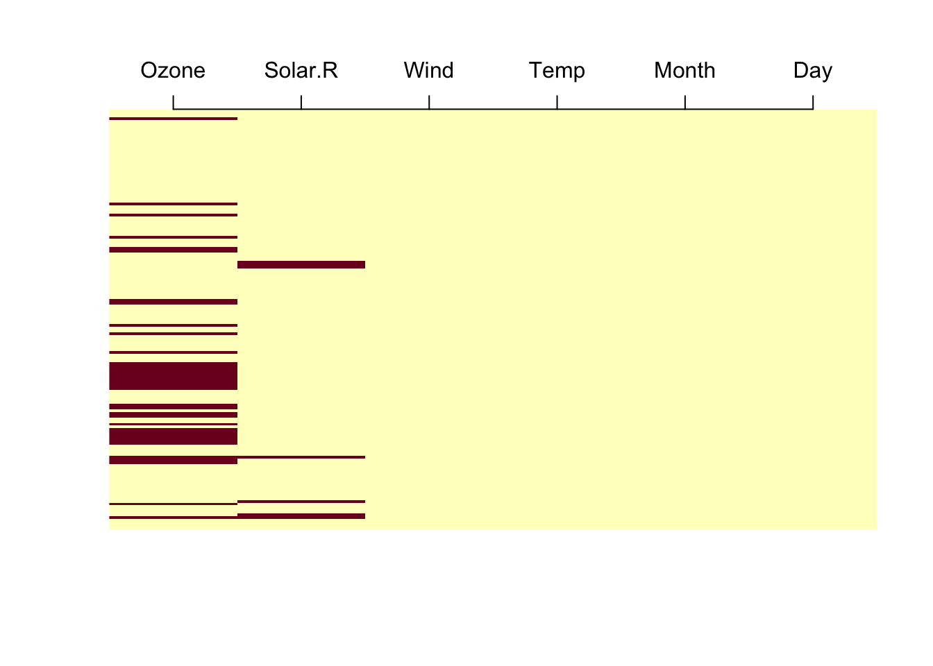
Missing value imputation by random forests

  Variables to impute:      Solar.R
  Variables used to impute: Ozone, Solar.R, Wind, Temp, Month, Day
iter 1: .
iter 2: .
iter 3: .
iter 4: .
iter 5: .

Missing value imputation by random forests

  Variables to impute:      Solar.R
  Variables used to impute: Ozone, Solar.R, Wind, Temp, Month, Day
iter 1: .
iter 2: .
iter 3: .

Missing value imputation by random forests

  Variables to impute:      Solar.R
  Variables used to impute: Ozone, Solar.R, Wind, Temp, Month, Day
iter 1: .
iter 2: .
iter 3: .

Missing value imputation by random forests

  Variables to impute:      Solar.R
  Variables used to impute: Ozone, Solar.R, Wind, Temp, Month, Day
iter 1: .
iter 2: .
iter 3: .
iter 4: .

Missing value imputation by random forests

  Variables to impute:      Solar.R
  Variables used to impute: Ozone, Solar.R, Wind, Temp, Month, Day
iter 1: .
iter 2: .
iter 3: .

Missing value imputation by random forests

  Variables to impute:      Solar.R
  Variables used to impute: Ozone, Solar.R, Wind, Temp, Month, Day
iter 1: .
iter 2: .
iter 3: .
iter 4: .
iter 5: .
iter 6: .

Missing value imputation by random forests

  Variables to impute:      Solar.R
  Variables used to impute: Ozone, Solar.R, Wind, Temp, Month, Day
iter 1: .
iter 2: .
iter 3: .

Missing value imputation by random forests

  Variables to impute:      Solar.R
  Variables used to impute: Ozone, Solar.R, Wind, Temp, Month, Day
iter 1: .
iter 2: .
iter 3: .
iter 4: .

Missing value imputation by random forests

  Variables to impute:      Solar.R
  Variables used to impute: Ozone, Solar.R, Wind, Temp, Month, Day
iter 1: .
iter 2: .
iter 3: .

Missing value imputation by random forests

  Variables to impute:      Solar.R
  Variables used to impute: Ozone, Solar.R, Wind, Temp, Month, Day
iter 1: .
iter 2: .
iter 3: .
iter 4: .
iter 5: .

Missing value imputation by random forests

  Variables to impute:      Solar.R
  Variables used to impute: Ozone, Solar.R, Wind, Temp, Month, Day
iter 1: .
iter 2: .
iter 3: .

Missing value imputation by random forests

  Variables to impute:      Solar.R
  Variables used to impute: Ozone, Solar.R, Wind, Temp, Month, Day
iter 1: .
iter 2: .
iter 3: .

Missing value imputation by random forests

  Variables to impute:      Solar.R
  Variables used to impute: Ozone, Solar.R, Wind, Temp, Month, Day
iter 1: .
iter 2: .
iter 3: .
iter 4: .

Missing value imputation by random forests

  Variables to impute:      Solar.R
  Variables used to impute: Ozone, Solar.R, Wind, Temp, Month, Day
iter 1: .
iter 2: .
iter 3: .

# fit 20 models
models <- lapply(airqualityMImp, function(x) lm(Ozone ~ Wind + Temp, x))

# use mice package to compute corrected p-values
require(mice)
summary(pooled_fit <- pool(models)) 

         term   estimate  std.error statistic       df      p.value
1 (Intercept) -71.033218 23.5779922 -3.012692 111.0406 3.207552e-03
2        Wind  -3.055491  0.6632503 -4.606844 111.0406 1.096691e-05
3        Temp   1.840179  0.2499634  7.361793 111.0406 3.377387e-11

More on missing data and imputation methods in Stef van Buuren’s book “Flexible Imputation of Missing Data”

library(mitools)

data(smi)
models<-with(smi, glm(drinkreg~wave*sex,family=binomial()))
summary(MIcombine(models))

Multiple imputation results:
      with(smi, glm(drinkreg ~ wave * sex, family = binomial()))
      MIcombine.default(models)
                results         se      (lower     upper) missInfo
(Intercept) -2.25974358 0.26830731 -2.78584855 -1.7336386      4 %
wave         0.24055250 0.06587423  0.11092461  0.3701804     12 %
sex          0.64905222 0.34919264 -0.03537187  1.3334763      1 %
wave:sex    -0.03725422 0.08609199 -0.20623121  0.1317228      7 %

Bhaskaran, Krishnan, and Liam Smeeth. 2014. “What Is the Difference Between Missing Completely at Random and Missing at Random?” International Journal of Epidemiology 43 (4): 1336–39.