12 Summary and concluding thoughts
12.1 Reminder: Modelling Strategy
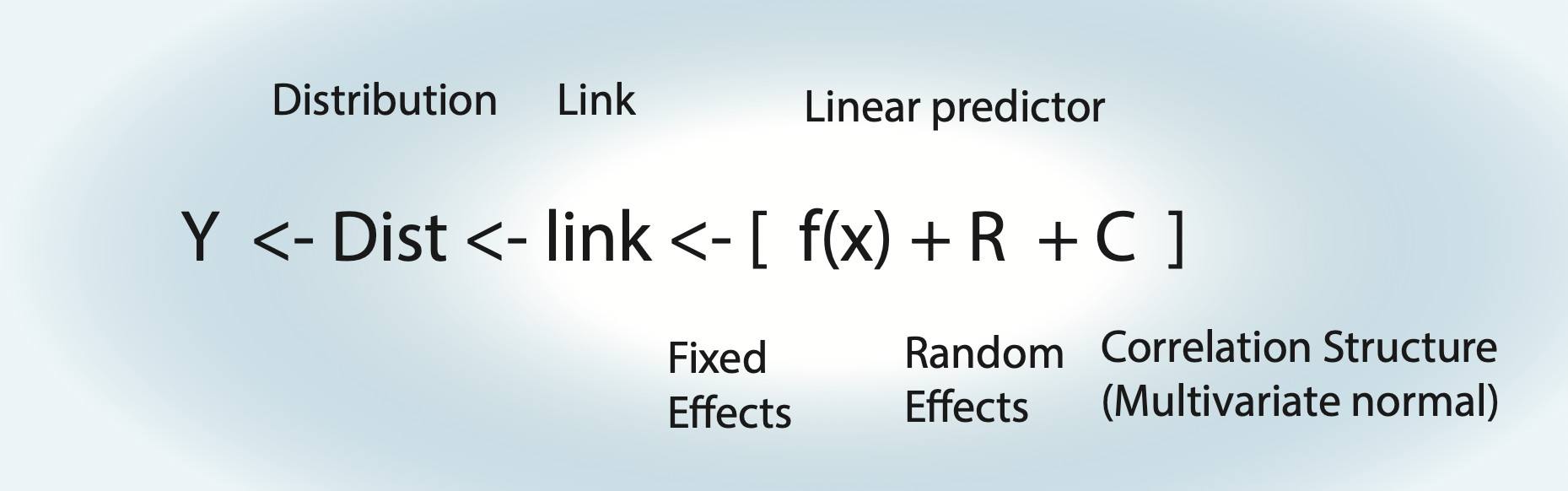
Things to note:
- For an lm, the link function is the identity function.
- Fixed effects \(\operatorname{f}(x)\) can be either a polynomial \(\left( a \cdot x = b \right)\) = linear regression, a nonlinear function = nonlinear regression, or a smooth spline = generalized additive model (GAM).
- Random effects assume normal distribution for groups.
- Random effects can also act on fixed effects (random slope).
- For an lm with correlation structure, C is integrated in Dist. For all other GLMMs, there is another distribution, plus the additional multivariate normal on the linear predictor.
Strategy for analysis:
- Define formula via scientific questions + confounders.
- Define type of GLM (lm, logistic, Poisson).
- Blocks in data -> Random effects, start with random intercept.
Fit this base model, then do residual checks for
- Wrong functional form -> Change fitted function.
- Wrong distribution-> Transformation or GLM adjustment.
- (Over)dispersion -> Variable dispersion GLM.
- Heteroskedasticity -> Model dispersion.
- Zero-inflation -> Add ZIP term.
- Correlation -> Add correlation structure.
And adjust the model accordingly.
Packages to fit thes models (see Apppedix: syntax cheat sheet):
baseR:lm,glm.lme4: mixed models,lmer,glmer.mgcv: GAM.nlme: Variance and correlations structure modelling for linear (mixed) models, usinggls+lme.glmmTMB: Generalized linear mixed models with variance / correlation modelling and zip term.
Alternatively, you could move to Bayesian estimates with brms, which allows all that, easier inclusion of shrinkage, and p-value / df problems less visible
12.2 Thoughts About the Analysis Pipeline
In statistics, we rarely use a simple analysis. We often use an entire pipeline, consisting, for example, of the protocol that I sketched in chapter @ref(protocol). What we should constantly ask ourselves: Is our pipeline good? By “good”, we typically mean: If 1000 analyses are run in that way:
- What is the typical error of the estimate?
- What is the Type I error (false positives)?
- Are the confidence intervals correctly calculated?
- …
The way to check this is to run simulations. For example, the following function creates data that follows the assumptions of a linear regression with slope 0.5, then fits a linear regression, and returns the estimate
getEstimate = function(n = 100){
  x = runif(n)
  y = 0.5 * x + rnorm(n)
  fit = lm(y ~ x)
  x = summary(fit)
  return(x$coefficients[2, 1])  # Get fitted x weight (should be ~0.5).
}
The replicate function allows us to execute this 1000 times:
set.seed(543210)

out = replicate(1000, getEstimate())
Plotting the result, we can check whether the linear regression is an unbiased estimator for the slope.
hist(out, breaks = 50)
abline(v = 0.5, col = "red")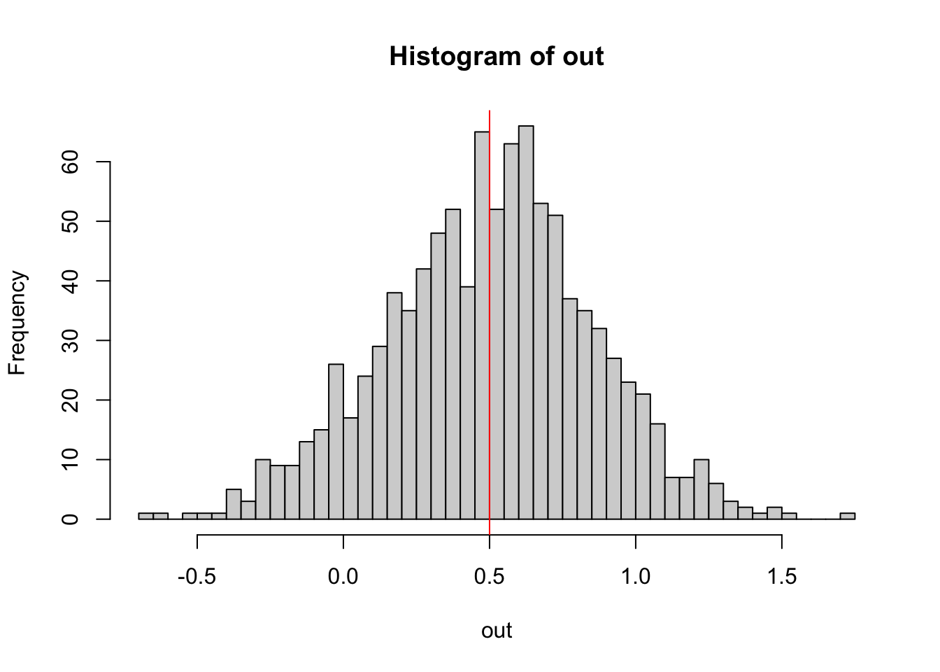
“Unbiased” means that, while each single estimate will have some error, the mean of many estimates will spread around the true value.
Explicitly calculating these values
Bias
mean(out) - 0.5 # Should be ~0.[1] -0.001826401Variance / standard deviation of the estimator
sd(out)[1] 0.3587717To check p-values, we could run:
set.seed(12345)

getEstimate = function(n = 100){  # Mind: Function has changed!
  x = runif(n)
  y = rnorm(n)  # No dependence of x! Identical: y = 0 * x + rnorm(100).
  fit = lm(y ~ x)
  x = summary(fit)
  return(x$coefficients[2, 4])  # P-value for H0: Weight of x = 0.
}

out = replicate(2000, getEstimate())

hist(out) # Expected: Uniformly distributed p-values. -> Check.
mean(out < 0.05) # Expected: ~0.05. But this is NO p-value... Check H0/H1![1] 0.0515# Explanation of syntax: Logical vectors are interpreted as vectors of 0s and 1s.To check the properties of other, possibly more complicated pipelines, statisticians will typically use the same technique. I recommend doing this! For example, you could modify the function above to have a non-normal error. How much difference does that make? Simulating often beats recommendations in the books!
12.3 Experimental design and power analysis
All we have learned in this course directly informs experimental and research design, may it be of controlled experiments, quasi-experiments or observational studies.
As a start, note our discussions of causality and model selection:
First of all, research design needs a goal: do you want to design for prediction or (causal) inference
If you are after causal inference, try to control confounders, and if not, try to measure them. It is often possible even in observational settings to control confounders, e.g. by selecting the observations in a way that confouders are at the same value. This can be useful because, as we discussed, adjusting for collinear variable is possible, but cost power.
In experimental settings, blocked designs where blocks will be later treated as a RE are standard
If you have decided on the selection of variables, treat your analysis as fixed. Perform a pilot study and/or a power analysis for the entire study [things to be added]