11  Machine Learning

The idea of machine learning is to maximize the predictive performance, which means to make predictions of y for new observations:

Let’s assume that part of the data is unknown (which will be our test data):

airquality = airquality[complete.cases(airquality),]
indices = sample.int(nrow(airquality), 50)
train = airquality[-indices,]
test = airquality[indices,]

We first train a model on the train data and then use the model make predictions for new data (test data):

model = lm(Ozone~., data = train)
predictions = predict(model, newdata = test)
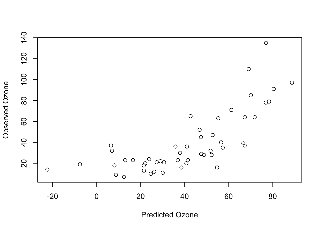
plot(predictions, test$Ozone, xlab = "Predicted Ozone", ylab = "Observed Ozone")

We can calculate the predictive performance (or prediction) error, for example, by using the correlation factor:

cor(predictions, test$Ozone)
## [1] 0.7507237
#R^2:
cor(predictions, test$Ozone)**2
## [1] 0.5635861

So the linear regression model is a great model for inferential statistics because it is interpretable (we exactly know how the variables are connected to the response). Many ML algorithms are not interpretable at all - they trade interpretability for predictive performance.

Random Forest is a famous algorithm which was first described by Leo Breiman, 2001. The idea of the random forest is to fit hundreds of ‘weak’ decision trees on bootstrap samples from the original data. Weak means that the decision trees are intentionally ‘constrained’ in their complexity (by random subsampling the set of features in each split):

library(randomForest)
## randomForest 4.7-1.1
## Type rfNews() to see new features/changes/bug fixes.
model = randomForest(Ozone~., data = train)
predictions = predict(model, newdata = test)
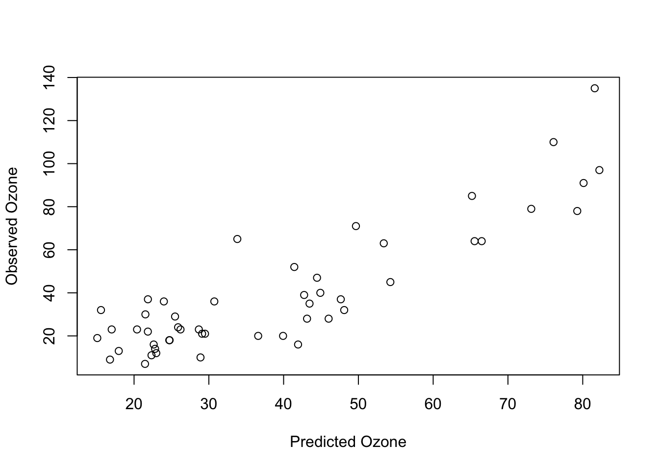
plot(predictions, test$Ozone, xlab = "Predicted Ozone", ylab = "Observed Ozone")

cor(predictions, test$Ozone)
## [1] 0.8743062
#R^2:
cor(predictions, test$Ozone)**2
## [1] 0.7644113

Our Random Forest achieved a higher predictive performance! BUT:

summary(model)
##                 Length Class  Mode     
## call              3    -none- call     
## type              1    -none- character
## predicted        61    -none- numeric  
## mse             500    -none- numeric  
## rsq             500    -none- numeric  
## oob.times        61    -none- numeric  
## importance        5    -none- numeric  
## importanceSD      0    -none- NULL     
## localImportance   0    -none- NULL     
## proximity         0    -none- NULL     
## ntree             1    -none- numeric  
## mtry              1    -none- numeric  
## forest           11    -none- list     
## coefs             0    -none- NULL     
## y                61    -none- numeric  
## test              0    -none- NULL     
## inbag             0    -none- NULL     
## terms             3    terms  call

…doesn’t tell us anything about effects or p-values. However, compared to other ML algorithms (e.g. artificial neural networks), at least the RF has a variable importance that reports which features were the most important features (similar to an ANOVA):

importance(model)
##         IncNodePurity
## Solar.R     13699.618
## Wind        17359.697
## Temp        20800.423
## Month        7436.931
## Day         12076.380

For the RF, the Temp was the most important feature, followed by Wind.

Tip

In ML a slightly different wording is used. Explanatory variables are called features. Datasets with responses with numerical values (e.g. Normal distribution or even Poisson distribution) are called regression tasks. Datasets with categorical responses (e.g. Binomial) are called classification tasks.

11.1 Regression

We call task with a numerical response variable a regression task:

indices = sample.int(nrow(airquality), 50)
train = airquality[-indices,]
test = airquality[indices,]

# 1. Fit model on train data:
model = randomForest(Ozone~., data = train)

# 2. Make Predictions
predictions = predict(model, newdata = test)

# 3. Compare predictions with observed values:
## the root mean squared error is commonly used as an error statistic:
sqrt(mean((predictions-test$Ozone)**2))
## [1] 20.41785
# Or use a correlationf actor
cor(predictions, test$Ozone)
## [1] 0.9017803
# Or Rsquared
cor(predictions, test$Ozone)**2
## [1] 0.8132077

11.2 Classification

We call a task with a categorical response variable a classification task (see also multi-class and multi-label classification):

indices = sample.int(nrow(iris), 50)
train = iris[-indices,]
test = iris[indices,]

# 1. Fit model on train data:
model = randomForest(Species~., data = train)

# 2. Make Predictions
predictions = predict(model, newdata = test)

# 3. Compare predictions with observed values:
mean(predictions == test$Species) # accuracy
## [1] 0.94

96% accuracy, which means only 4% of the observations were wrongly classified by our random forest!

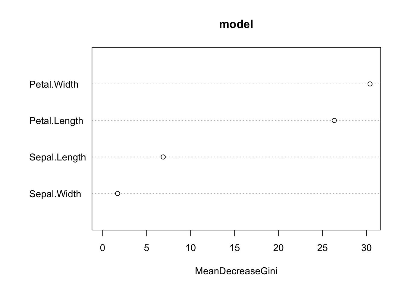
Variable importance:

varImpPlot(model)

Petal.Width and Petal.Length were the most important predictors!