Xobs = rnorm(n = 100, mean = 0, sd = 1.0)8 Simple linear regression
In this chapter, you will:
- perform simple linear regression for numeric and categorical predictors
- interpret regression outputs
- check the residuals of regression models
8.1 Maximum Likelihood Estimator
\(likelihood = P(D|model, parameter)\)
The likelihood is the probability to observe the Data given a certain model (which is described by its parameter).
It is an approach to optimize a model/parameter to find the set of parameters that describes best the observed data.
A simple example: we want to estimate the average of a random vector and we assume that our model is a normal distribution (so we assume that the data originated from a normal distribution). We want to optimize the two parameters that describe the normal distribution: the mean, and the standard deviation:
Let’s create the “oberved” vector:
Now, we assume that the mean and the standard deviation of the vector is unknown and we want to find them. Let’s write the likelihood function (in reality, we use logLikelihood for numerical reasons):
likelihood = function(par) { # we give two parameters, mean and sd
  # calculate for each observation to observe the data given our model:
  lls = dnorm(Xobs, mean = par[1], sd = par[2], log = TRUE)
  # we use the logLikilihood for numerical reasons
  return(sum(lls))
}
Let’s guess some values for the mean and sd and see what the function returns
likelihood(c(0, 0.2))
## [1] -1274.247
This number alone doens’t tell us much, we have com compare many different guesses to see which combination of parameters gives is the most plausible. To make it easier to understand, we will fix the sd in 1 and plot how the likelihood changes with changing the mean:
likelihood_mean = function(mean.par){
  likelihood(c(mean.par, 1.0))}

plot(seq(-5, 5.0, length.out = 100),
     sapply(seq(-5, 5.0, length.out = 100), likelihood_mean),
     xlab = 'Different mean values',
     ylab = "negative logLikelihood")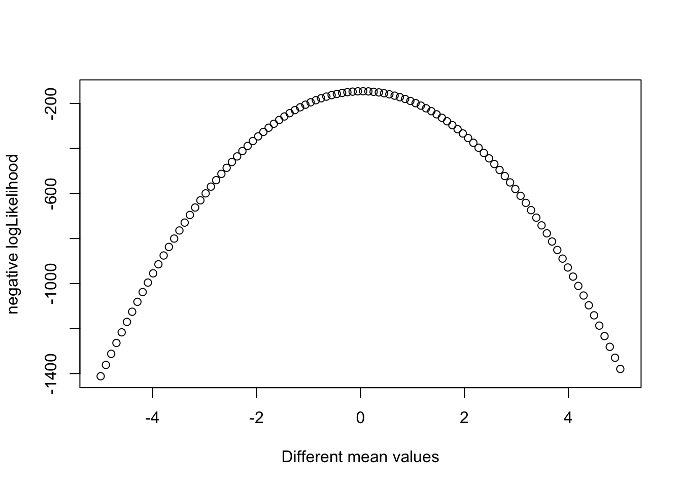
The optimum (highest peak) is at 0, which corresponds to the mean we used to sample Xobs. We could do the same with the sd - fix the mean and vary the sd to find it.
However it is tedious to try all values manually to find the best value, especially if we have to optimize several parameters. For that, we can use an optimizer in R which finds for us the best set of parameters:
opt = optim(c(0.0, 1.0), fn = function(par) -likelihood(par), hessian = TRUE )We can use the shape of the likelihood to calculate standard errors for our estimates:
st_errors = sqrt(diag(solve(opt$hessian)))With that we can calculate the confidence interval for our estimates. When the estimator is repeatedly used, 95% of the calculated confidence intervals will include the true value!
cbind(opt$par-1.96*st_errors, opt$par+1.96*st_errors)
##            [,1]      [,2]
## [1,] -0.1706372 0.2355346
## [2,]  0.8925465 1.1797585
In short, if we would do a t.test for our Xobs (to test whether the mean is stat. significant different from zero), the test would be non significant, and a strong indicator for that is when the 0 is within the confidence interval. Let’s compare our CI to the one calculated by the t-test:
t.test(Xobs)
##
##  One Sample t-test
##
## data:  Xobs
## t = 0.31224, df = 99, p-value = 0.7555
## alternative hypothesis: true mean is not equal to 0
## 95 percent confidence interval:
##  -0.1741130  0.2391426
## sample estimates:
##  mean of x
## 0.03251482
The results are lmost the same! The t-test also calculates the MLE to get the standard error and the confidence interval.
8.2 The theory of linear regression
If we want to test for an association between two continuous variables, we can calculate the correlation between the two - and with the cor.test function we can test even for significance. But, the correlation doesn’t report the magnitude, the strength, of the effect:
X = runif(100)
par(mfrow = c(1,1))
plot(X, 0.5*X, ylim = c(0, 1), type = "p", pch = 15, col = "red", xlab = "X", ylab = "Y")
points(X, 1.0*X, ylim = c(0, 1), type = "p", pch = 15, col = "blue", xlab = "X", ylab = "Y")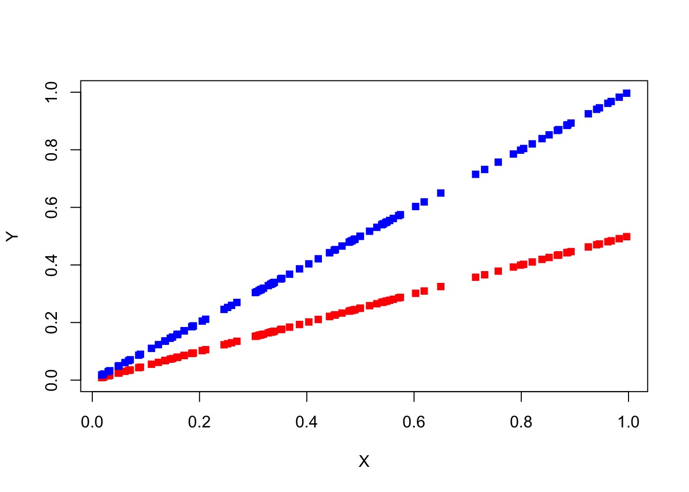
cor(X, 0.5*X)
## [1] 1
cor(X, 1.0*X)
## [1] 1
Both have a correlation factor of 1.0! But we see clearly that the blue line has an stronger effect on Y then the red line.
Solution: Linear regression models
They describe the relationship between a dependent variable and one or more explanatory variables:
\[ y = a_0 +a_1*x \]
(x = explanatory variable; y = dependent variable; a0=intercept; a1= slope)
Examples:
plot(X, 0.5*X, ylim = c(0, 1), type = "p", pch = 16, col = "black", xlab = "X", ylab = "Y", lwd = 1.5)
points(X, 0.5*X, col = "red", type = "l", lwd = 1.5)
points(X, 1.0*X, ylim = c(0, 1), type = "p", pch = 16, col = "black", xlab = "X", ylab = "Y", lwd = 1.5)
points(X, 1.0*X, ylim = c(0, 1), type = "l", pch = 16, col = "blue", xlab = "X", ylab = "Y", lwd = 1.5)
legend("topleft", col = c("red", "blue"), lty = 1,legend = c('Y = 0.5*X+0', 'Y = 1.0**X+0'))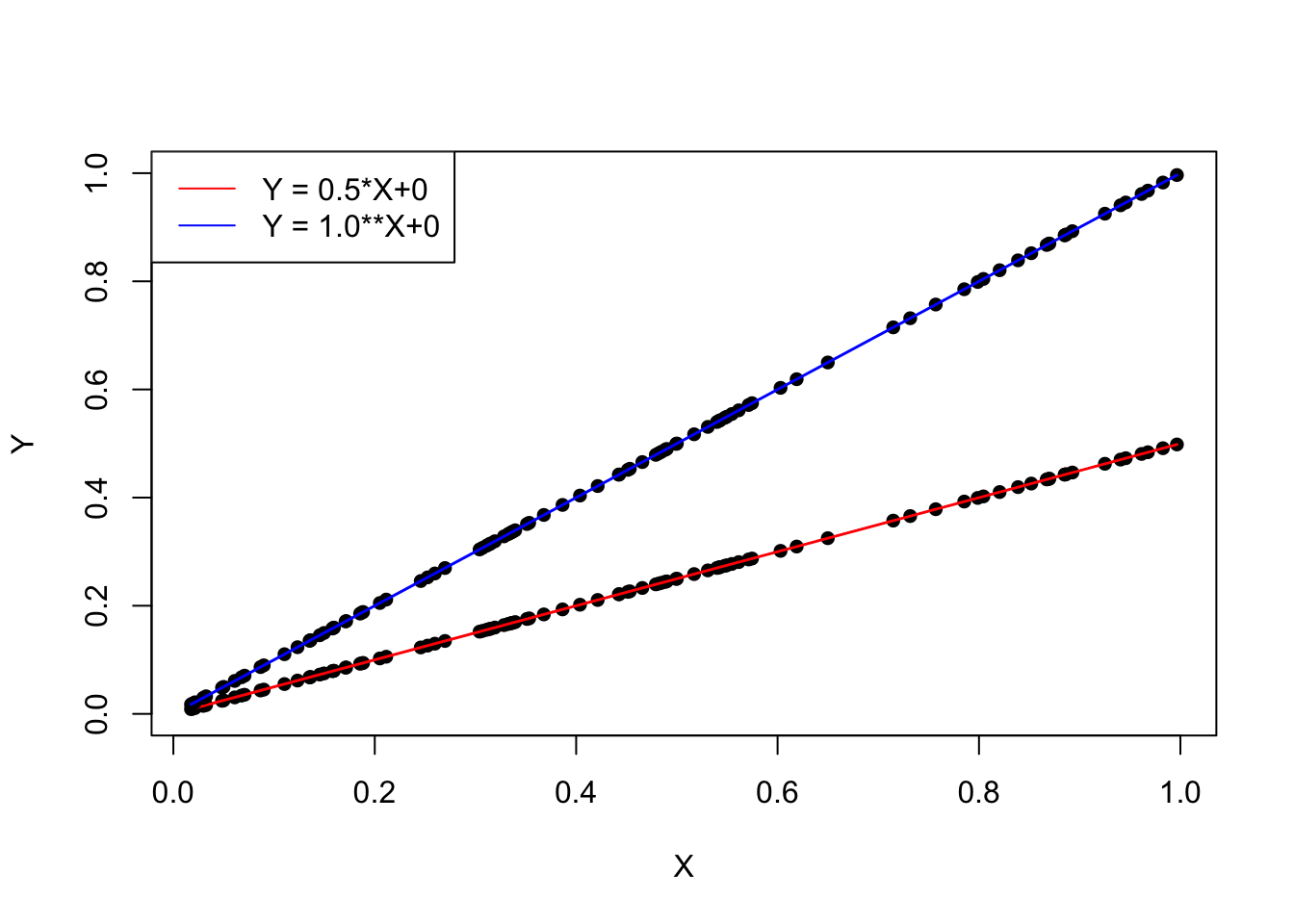
We can get the parameters (slope and intercept) with the MLE. However, we need first to make another assumptions, usually the model line doesn’t perfectly the data because there is an observational error on Y, so the points scatter around the line:
plot(X, 0.5*X+rnorm(100, sd = 0.05), ylim = c(0, 1), type = "p", pch = 16, col = "black", xlab = "X", ylab = "Y", lwd = 1.5)
points(X, 0.5*X, col = "red", type = "l", lwd = 1.5)
points(X, 1.0*X+rnorm(100, sd = 0.05), ylim = c(0, 1), type = "p", pch = 16, col = "black", xlab = "X", ylab = "Y", lwd = 1.5)
points(X, 1.0*X, ylim = c(0, 1), type = "l", pch = 16, col = "blue", xlab = "X", ylab = "Y", lwd = 1.5)
legend("topleft", col = c("red", "blue"), lty = 1,legend = c('Y = 0.5*X+0', 'Y = 1.0**X+0'))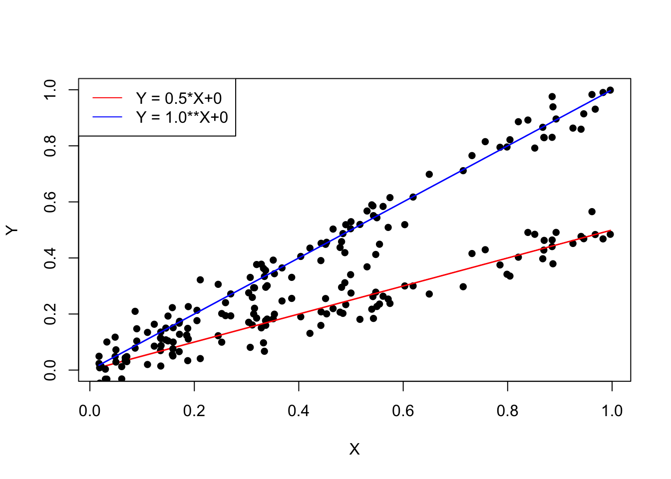
And the model extends to:
\[ y = a_0 + a_1*x +\epsilon, \epsilon \sim N(0, sd) \]
Which we can also rewrite into:
\[ y = N(a_0 + a_1*x, sd) \]
Which is very similar to our previous MLE, right? The only difference is now that the mean depends now on x, let’s optimize it again:
Xobs = rnorm(100, sd = 1.0)
Y = Xobs + rnorm(100,sd = 0.2)
likelihood = function(par) { # three parameters now
  lls = dnorm(Y, mean = Xobs*par[2]+par[1], sd = par[3], log = TRUE) # calculate for each observation the probability to observe the data given our model
  # we use the logLikilihood because of numerical reasons
  return(sum(lls))
}

likelihood(c(0, 0, 0.2))
## [1] -1162.229
opt = optim(c(0.0, 0.0, 1.0), fn = function(par) -likelihood(par), hessian = TRUE )

opt$par
## [1] 0.002927292 0.997608527 0.216189328
Our true parameters are 0.0 for the intercept, 1.0 for the slope, and 0.22 for the sd of the observational error.
Now, we want to test whether the effect (slope) is statistically significant different from 0:
- calculate standard error
- calculate t-statistic
- calculate p-value
st_errors = sqrt(diag(solve(opt$hessian)))
st_errors[2]
## [1] 0.02226489
t_statistic = opt$par[2] / st_errors[2]
pt(t_statistic, df = 100-3, lower.tail = FALSE)*2
## [1] 1.264962e-66
The p-value is smaller than \(\alpha\), so the effect is significant! However, it would be tedious to do that always by hand, and because it is probably one of the most used analysis, there’s a function for it in R:
model = lm(Y~Xobs) # 1. Get estimates, MLE
model
##
## Call:
## lm(formula = Y ~ Xobs)
##
## Coefficients:
## (Intercept)         Xobs
##    0.002927     0.997569
summary(model) # 2. Calculate standard errors, CI, and p-values
##
## Call:
## lm(formula = Y ~ Xobs)
##
## Residuals:
##      Min       1Q   Median       3Q      Max
## -0.49919 -0.13197 -0.01336  0.14239  0.64505
##
## Coefficients:
##             Estimate Std. Error t value Pr(>|t|)
## (Intercept) 0.002927   0.021838   0.134    0.894
## Xobs        0.997569   0.022490  44.355   <2e-16 ***
## ---
## Signif. codes:  0 '***' 0.001 '**' 0.01 '*' 0.05 '.' 0.1 ' ' 1
##
## Residual standard error: 0.2184 on 98 degrees of freedom
## Multiple R-squared:  0.9526, Adjusted R-squared:  0.9521
## F-statistic:  1967 on 1 and 98 DF,  p-value: < 2.2e-16
8.3 Understanding the linear regression
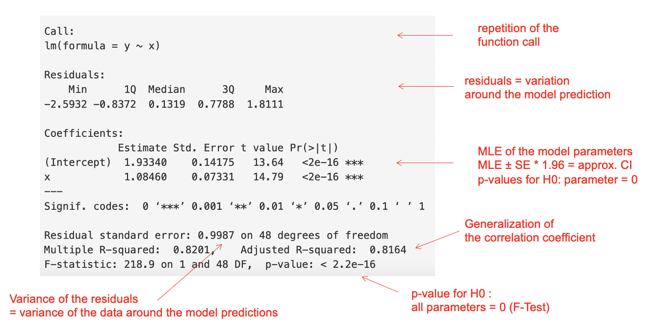
Besides the MLE, there are also several tests in a regression. The most important are
significance of each parameter. t-test: H0 = variable has no effect, that means the estimator for the parameter is 0
significance of the model. F-test: H0 = none of the explanatory variables has an effect, that means all estimators are 0
Example:
pairs(airquality)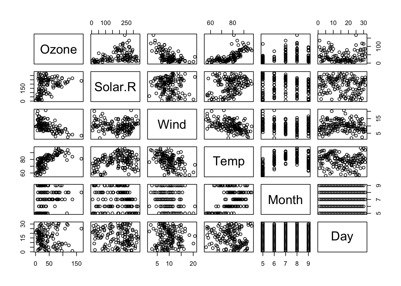
# first think about what is explanatory / predictor
# and what is the dependent variable (e.g. in Ozone and Temp)

# par(mfrow = c(1, 1))
plot(Ozone ~ Temp, data = airquality)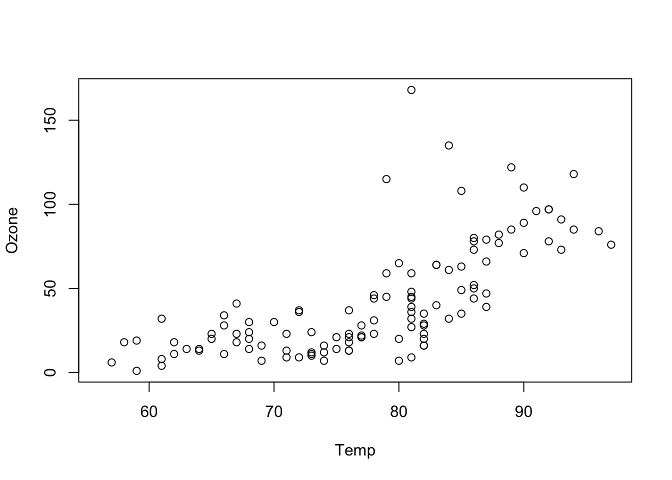
fit1 = lm(Ozone ~ Temp, data = airquality)
summary(fit1)
##
## Call:
## lm(formula = Ozone ~ Temp, data = airquality)
##
## Residuals:
##     Min      1Q  Median      3Q     Max
## -40.729 -17.409  -0.587  11.306 118.271
##
## Coefficients:
##              Estimate Std. Error t value Pr(>|t|)
## (Intercept) -146.9955    18.2872  -8.038 9.37e-13 ***
## Temp           2.4287     0.2331  10.418  < 2e-16 ***
## ---
## Signif. codes:  0 '***' 0.001 '**' 0.01 '*' 0.05 '.' 0.1 ' ' 1
##
## Residual standard error: 23.71 on 114 degrees of freedom
##   (37 observations deleted due to missingness)
## Multiple R-squared:  0.4877, Adjusted R-squared:  0.4832
## F-statistic: 108.5 on 1 and 114 DF,  p-value: < 2.2e-16
# gives a negative values for the intercept = negative Ozone levels when Temp = 0
# this does not make sense (>extrapolation)

# we can also fit a model without intercept,
# without means: intercept = 0; y = a*x
# although this doesn't make much sense here
fit2 = lm(Ozone ~ Temp - 1, data = airquality)
summary(fit2)
##
## Call:
## lm(formula = Ozone ~ Temp - 1, data = airquality)
##
## Residuals:
##    Min     1Q Median     3Q    Max
## -38.47 -23.26 -12.46  15.15 121.96
##
## Coefficients:
##      Estimate Std. Error t value Pr(>|t|)
## Temp  0.56838    0.03498   16.25   <2e-16 ***
## ---
## Signif. codes:  0 '***' 0.001 '**' 0.01 '*' 0.05 '.' 0.1 ' ' 1
##
## Residual standard error: 29.55 on 115 degrees of freedom
##   (37 observations deleted due to missingness)
## Multiple R-squared:  0.6966, Adjusted R-squared:  0.6939
## F-statistic:   264 on 1 and 115 DF,  p-value: < 2.2e-16

plot(Ozone ~ Temp, data = airquality, xlim = c(0,100), ylim = c(-150, 150))
abline(fit1, col = "green")
abline(fit2, col = "red", lty = 2)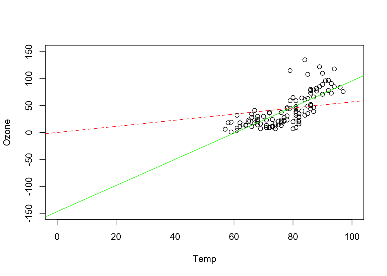
# there is no need to check normality of Ozone
hist(airquality$Ozone) # this is not normal, and that's no problem !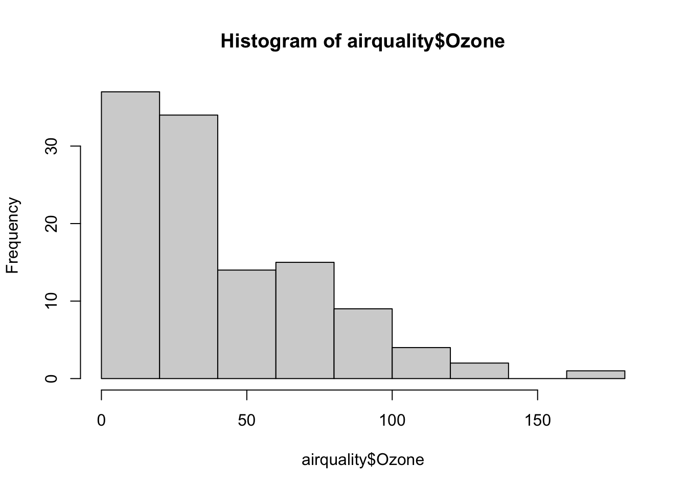
8.3.1 Model diagnostics
The regression optimizes the parameters under the condition that the model is correct (e.g. there is really a linear relationship). If the model is not specified correctly, the parameter values are still estimated - to the best of the model’s ability, but the result will be misleading, e.g. p-values and effect sizes
What could be wrong:
- the distribution (e.g. error not normal)
- the shape of the relationship between explanatory variable and dependent variable (e.g., could be non-linear)
The model’s assumptions must always be checked!
We can check the model by looking at the residuals (which are observed - predicted values) which should be normally distributed and should show no patterns:
X = runif(50)
Y = X + rnorm(50, sd = 0.2)
fit = lm(Y~X)
par(mfrow = c(1, 3))
plot(X, Y)
abline(fit, col = "red")
plot(X, Y - predict(fit), ylab = "Residuals")
abline(h = 0, col = "red")
hist(Y - predict(fit), main = "", xlab = "Residuals")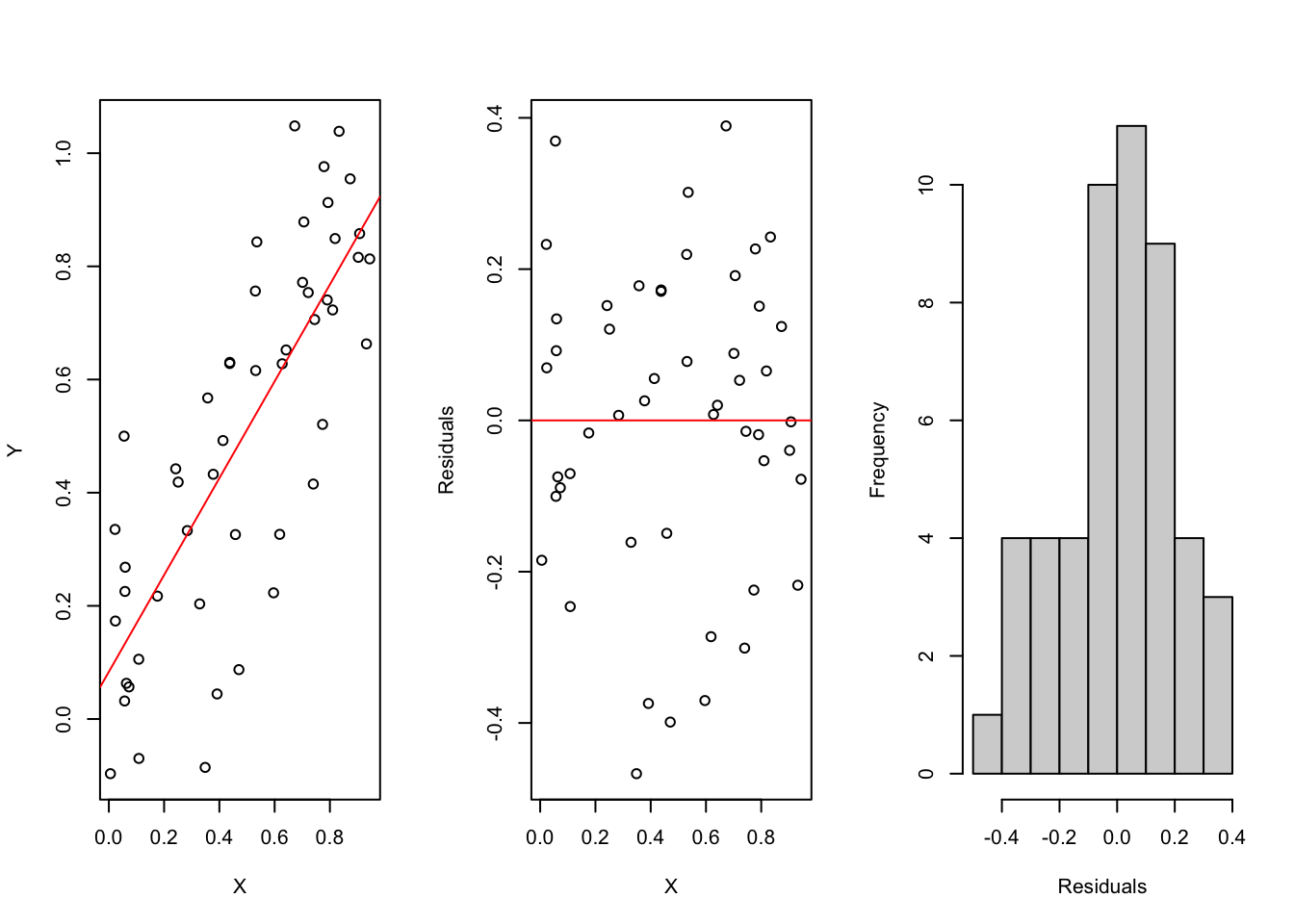
par(mfrow = c(1,1))The residuals should match the model assumptions. For linear regression:
- normal distribution
- constant variance
- independence of the data points
Example:
fit1 = lm(Ozone~Temp, data = airquality)
residuals(fit1)
##           1           2           3           4           6           7
##  25.2723695   8.1288530 -20.7285536  14.4158861  14.7010729  12.1297762
##           8           9          11          12          13          14
##  22.7019960   6.8445894 -25.7285536  -4.5850371  -2.2989271  -4.1563338
##          15          16          17          18          19          20
##  24.1306993   5.5584795  20.7010729  14.5594026  11.8436662   7.4158861
##          21          22          23          24          28          29
##   4.7019960 -19.2998503   2.8445894  30.8445894   7.2723695  -4.7294767
##          30          31          38          40          41          44
##  70.1279299  -0.5859602 -23.1581800  -0.5878065 -25.3016966 -29.1581800
##          47          48          49          50          51          62
## -19.0146635   9.1288530   9.1297762 -18.2998503 -24.5859602  77.9844134
##          63          64          66          67          68          69
## -10.4442899 -17.7294767   9.4131167 -14.5868833  10.2696001  20.5547869
##          70          71          73          74          76          77
##  20.5547869  15.8408968 -20.2998503 -22.7294767 -40.3007734  -1.7294767
##          78          79          80          81          82          85
## -17.1581800   3.9844134  14.6983034   3.5557101 -16.7285536  18.1270068
##          86          87          88          89          90          91
##  48.5557101 -32.1581800  -9.8729932  15.2696001 -11.8729932   9.4131167
##          92          93          94          95          96          97
##   9.2705233 -10.7294767 -40.7294767 -36.1581800  16.1270068 -24.4442899
##          98          99         100         101         104         105
##   1.6983034  52.8408968  17.4121935  38.4121935 -17.8729932 -24.1581800
##         106         108         109         110         111         112
##  17.6992266 -18.0146635  14.1279299 -14.5859602 -11.4433668   1.5566332
##         113         114         116         117         118         120
## -19.0146635 -18.8711470   0.1279299 118.2705233  11.1270068 -12.5887296
##         121         122         123         124         125         126
##  36.6973803  -2.1600263   3.6973803  21.9834902   1.5547869  -5.8739164
##         127         128         129         130         131         132
##  12.1260836 -17.3016966 -25.0155866 -27.3007734 -19.4433668 -14.1572569
##         133         134         135         136         137         138
##  -6.2998503  -5.7294767 -16.5859602 -12.0146635 -16.4424437 -12.4424437
##         139         140         141         142         143         144
##   3.5566332   2.2723695 -24.5859602   5.8436662 -36.1581800   4.5584795
##         145         146         147         148         149         151
##  -2.4424437 -13.7294767 -13.5850371   7.9871828   6.9862596 -21.1572569
##         152         153
## -19.5859602   1.8436662
hist(residuals(fit1))
# residuals are not normally distributed
# we do not use a test for this, but instead look at the residuals visually

# let's plot residuals versus predictor
plot(airquality$Temp[!is.na(airquality$Ozone)], residuals(fit1))
# model checking plots
oldpar= par(mfrow = c(2,2))
plot(fit1)
par(oldpar)
#> there's a pattern in the residuals > the model does not fit very well!
8.4 Linear regression with a categorical variable
We can also use categorical variables as an explanatory variable:
m = lm(weight~group, data = PlantGrowth)
summary(m)
##
## Call:
## lm(formula = weight ~ group, data = PlantGrowth)
##
## Residuals:
##     Min      1Q  Median      3Q     Max
## -1.0710 -0.4180 -0.0060  0.2627  1.3690
##
## Coefficients:
##             Estimate Std. Error t value Pr(>|t|)
## (Intercept)   5.0320     0.1971  25.527   <2e-16 ***
## grouptrt1    -0.3710     0.2788  -1.331   0.1944
## grouptrt2     0.4940     0.2788   1.772   0.0877 .
## ---
## Signif. codes:  0 '***' 0.001 '**' 0.01 '*' 0.05 '.' 0.1 ' ' 1
##
## Residual standard error: 0.6234 on 27 degrees of freedom
## Multiple R-squared:  0.2641, Adjusted R-squared:  0.2096
## F-statistic: 4.846 on 2 and 27 DF,  p-value: 0.01591
The lm estimates an effect/intercept for each level in the categorical variable. The first level of the categorical variable is used as a reference, i.e. the true effect for grouptrt1 is Intercept+grouptrt1 = 4.661 and grouptrt2 is 5.5242. Moreover, the lm tests for a difference of the reference to the other levels. So with this model we know whether the control is significant different from treatment 1 and 2 but we cannot say anything about the difference between trt1 and trt2.
If we are interested in testing trt1 vs trt2 we can, for example, change the reference level of our variable:
tmp = PlantGrowth
tmp$group = relevel(tmp$group, ref = "trt1")
m = lm(weight~group, data = tmp)
summary(m)
##
## Call:
## lm(formula = weight ~ group, data = tmp)
##
## Residuals:
##     Min      1Q  Median      3Q     Max
## -1.0710 -0.4180 -0.0060  0.2627  1.3690
##
## Coefficients:
##             Estimate Std. Error t value Pr(>|t|)
## (Intercept)   4.6610     0.1971  23.644  < 2e-16 ***
## groupctrl     0.3710     0.2788   1.331  0.19439
## grouptrt2     0.8650     0.2788   3.103  0.00446 **
## ---
## Signif. codes:  0 '***' 0.001 '**' 0.01 '*' 0.05 '.' 0.1 ' ' 1
##
## Residual standard error: 0.6234 on 27 degrees of freedom
## Multiple R-squared:  0.2641, Adjusted R-squared:  0.2096
## F-statistic: 4.846 on 2 and 27 DF,  p-value: 0.01591
Another example:
library(effects)
## Carregando pacotes exigidos: carData
## lattice theme set by effectsTheme()
## See ?effectsTheme for details.
library(jtools)

summary(chickwts)
##      weight             feed
##  Min.   :108.0   casein   :12
##  1st Qu.:204.5   horsebean:10
##  Median :258.0   linseed  :12
##  Mean   :261.3   meatmeal :11
##  3rd Qu.:323.5   soybean  :14
##  Max.   :423.0   sunflower:12

plot(weight ~ feed, chickwts)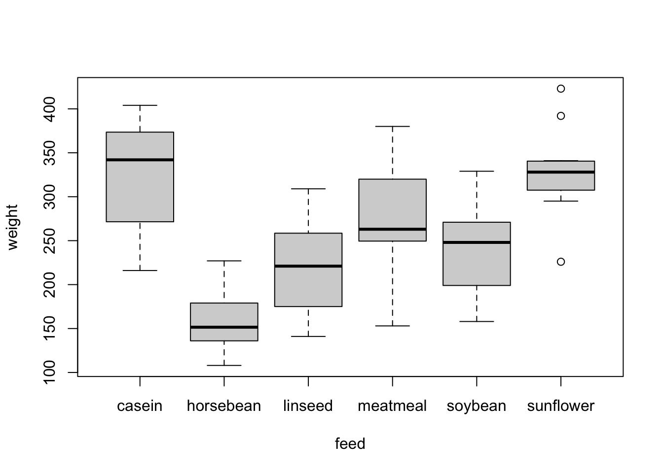
fit4 = lm(weight ~ feed, chickwts)

summary(fit4)
##
## Call:
## lm(formula = weight ~ feed, data = chickwts)
##
## Residuals:
##      Min       1Q   Median       3Q      Max
## -123.909  -34.413    1.571   38.170  103.091
##
## Coefficients:
##               Estimate Std. Error t value Pr(>|t|)
## (Intercept)    323.583     15.834  20.436  < 2e-16 ***
## feedhorsebean -163.383     23.485  -6.957 2.07e-09 ***
## feedlinseed   -104.833     22.393  -4.682 1.49e-05 ***
## feedmeatmeal   -46.674     22.896  -2.039 0.045567 *
## feedsoybean    -77.155     21.578  -3.576 0.000665 ***
## feedsunflower    5.333     22.393   0.238 0.812495
## ---
## Signif. codes:  0 '***' 0.001 '**' 0.01 '*' 0.05 '.' 0.1 ' ' 1
##
## Residual standard error: 54.85 on 65 degrees of freedom
## Multiple R-squared:  0.5417, Adjusted R-squared:  0.5064
## F-statistic: 15.36 on 5 and 65 DF,  p-value: 5.936e-10
anova(fit4) #get overall effect of feeding treatment
## Analysis of Variance Table
##
## Response: weight
##           Df Sum Sq Mean Sq F value    Pr(>F)
## feed       5 231129   46226  15.365 5.936e-10 ***
## Residuals 65 195556    3009
## ---
## Signif. codes:  0 '***' 0.001 '**' 0.01 '*' 0.05 '.' 0.1 ' ' 1

plot(allEffects(fit4))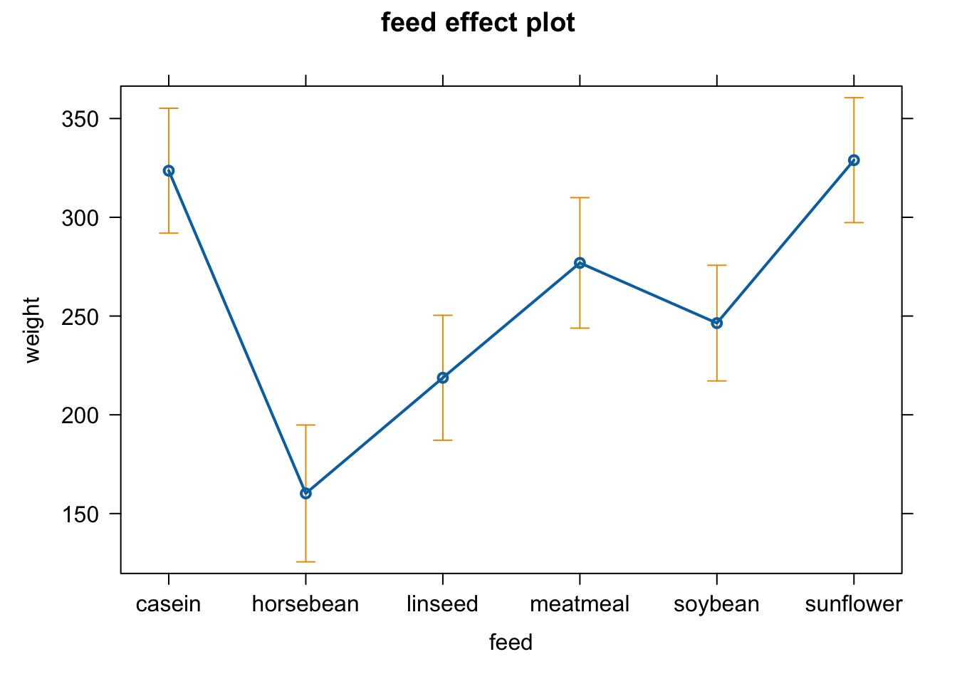
plot(allEffects(fit4, partial.residuals = T))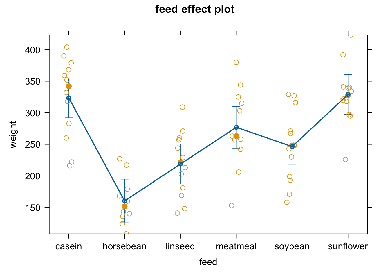
effect_plot(fit4, pred = feed, interval = TRUE, plot.points = F)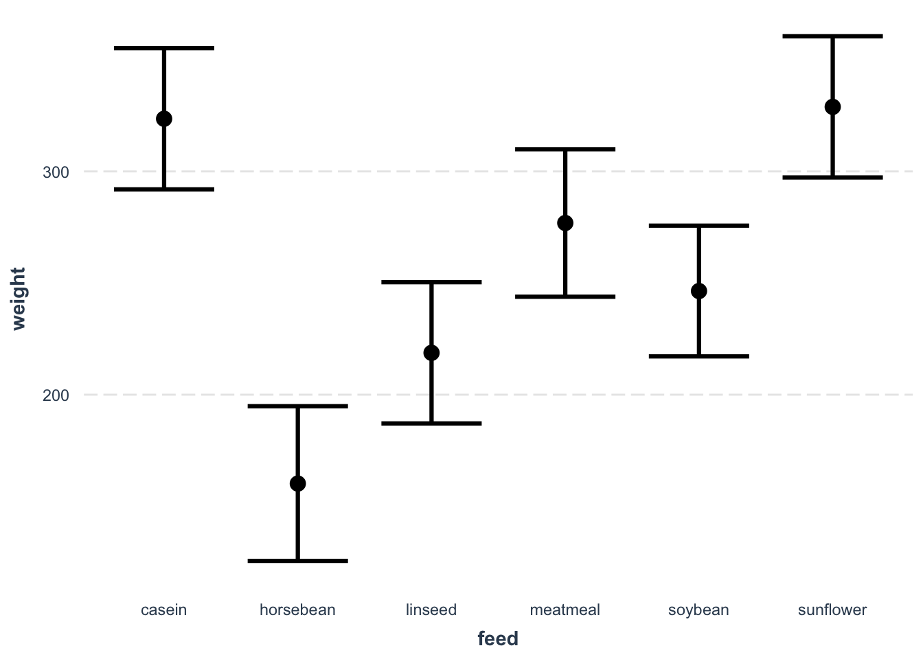
old.par = par(mfrow = c(2, 2))
plot(fit4)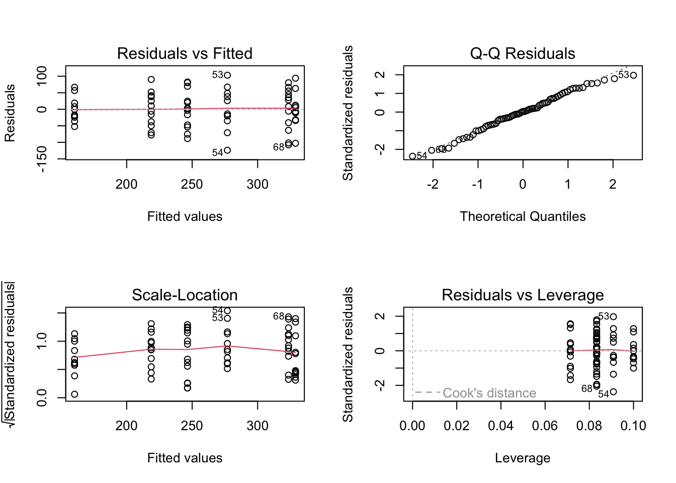
par(old.par)

boxplot(residuals(fit4) ~ chickwts$feed)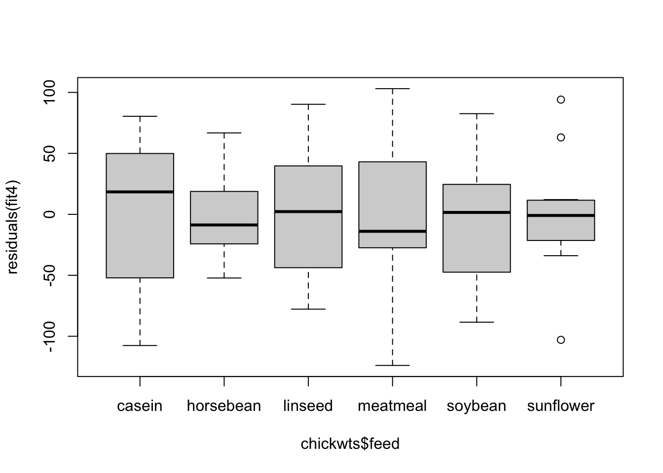
8.4.1 Linear regression with a quadratic term
What does simple linear regression mean?
simple = one predictor!
linear = linear in the parameters
If we add a quadratic term, this is still a linear combination: this is called polynomial.
\[ a0 + a1 * x + a2 * x^2 \]
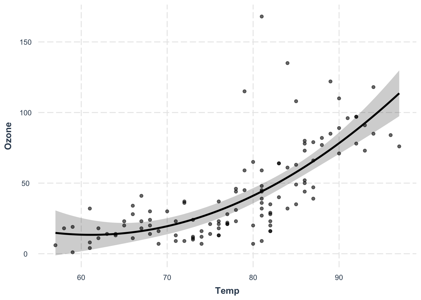
Le’ts model Ozone as a function of temperature and it’s quadratic term:
fit3 = lm(Ozone ~ Temp + I(Temp^2), data = airquality)
summary(fit3)
##
## Call:
## lm(formula = Ozone ~ Temp + I(Temp^2), data = airquality)
##
## Residuals:
##     Min      1Q  Median      3Q     Max
## -37.619 -12.513  -2.736   9.676 123.909
##
## Coefficients:
##              Estimate Std. Error t value Pr(>|t|)
## (Intercept) 305.48577  122.12182   2.501 0.013800 *
## Temp         -9.55060    3.20805  -2.977 0.003561 **
## I(Temp^2)     0.07807    0.02086   3.743 0.000288 ***
## ---
## Signif. codes:  0 '***' 0.001 '**' 0.01 '*' 0.05 '.' 0.1 ' ' 1
##
## Residual standard error: 22.47 on 113 degrees of freedom
##   (37 observations deleted due to missingness)
## Multiple R-squared:  0.5442, Adjusted R-squared:  0.5362
## F-statistic: 67.46 on 2 and 113 DF,  p-value: < 2.2e-16

oldpar= par(mfrow = c(2,2))
plot(fit3)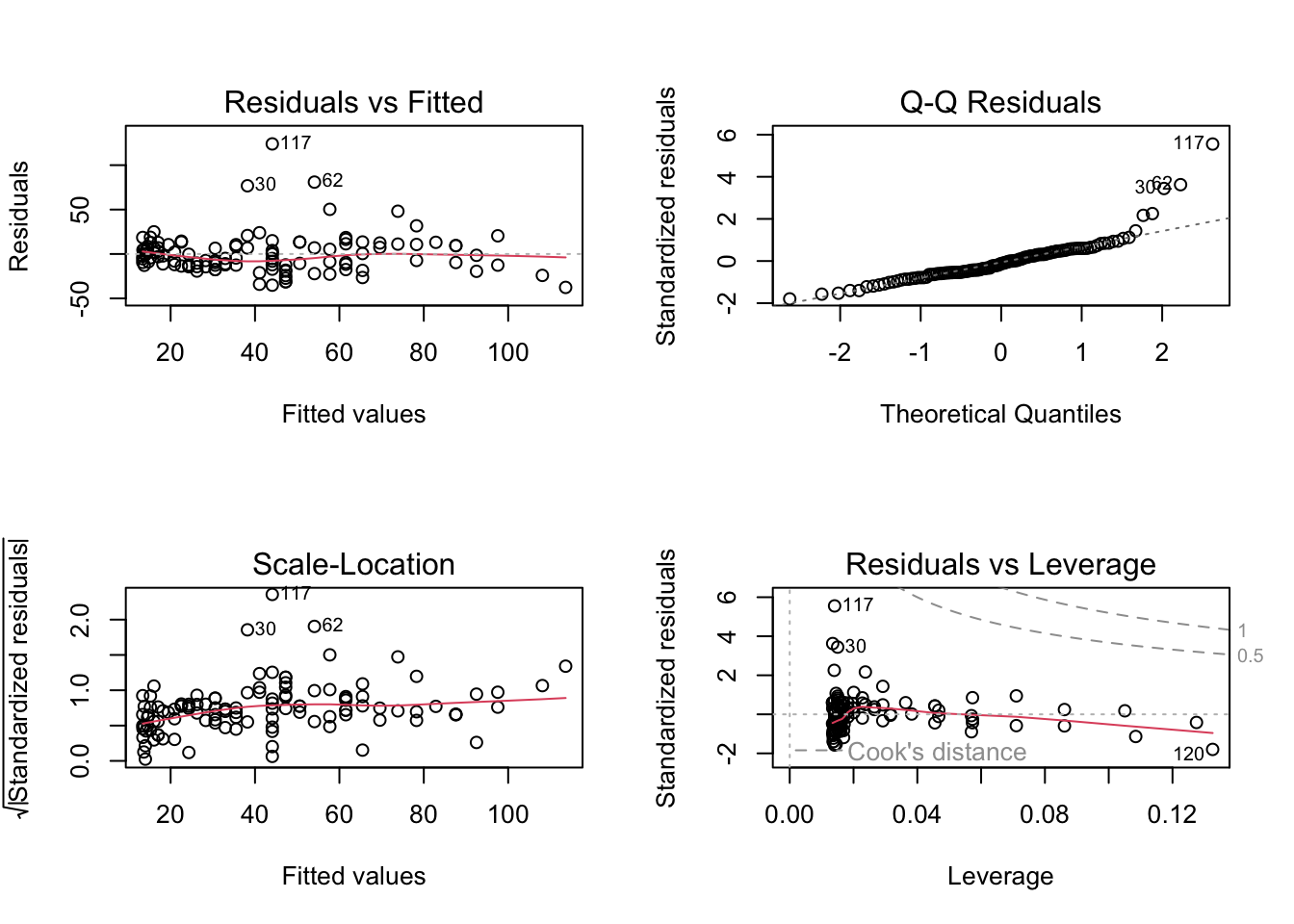
par(oldpar)Residual vs. fitted looks okay, but Outliers are still there, and additionally too wide. But for now, let’s plot prediction with uncertainty (plot line plus confidence interval):
OBS: If the relationship between x and y is not linear, we cannot use abline instead we predict values of x for different values of y based on the model:
plot(Ozone ~ Temp, data = airquality)
newDat = data.frame(Temp = 55:100)
predictions = predict(fit3, newdata = newDat, se.fit = T)
# and plot these into our figure:
lines(newDat$Temp, predictions$fit, col= "red")
# let's also plot the confidence intervals:
lines(newDat$Temp, predictions$fit + 1.96*predictions$se.fit, col= "red", lty = 2)
lines(newDat$Temp, predictions$fit - 1.96*predictions$se.fit, col= "red", lty = 2)

# add a polygon (shading for confidence interval)
x = c(newDat$Temp, rev(newDat$Temp))
y = c(predictions$fit - 1.96*predictions$se.fit,
      rev(predictions$fit + 1.96*predictions$se.fit))

polygon(x,y, col="#99009922", border = F )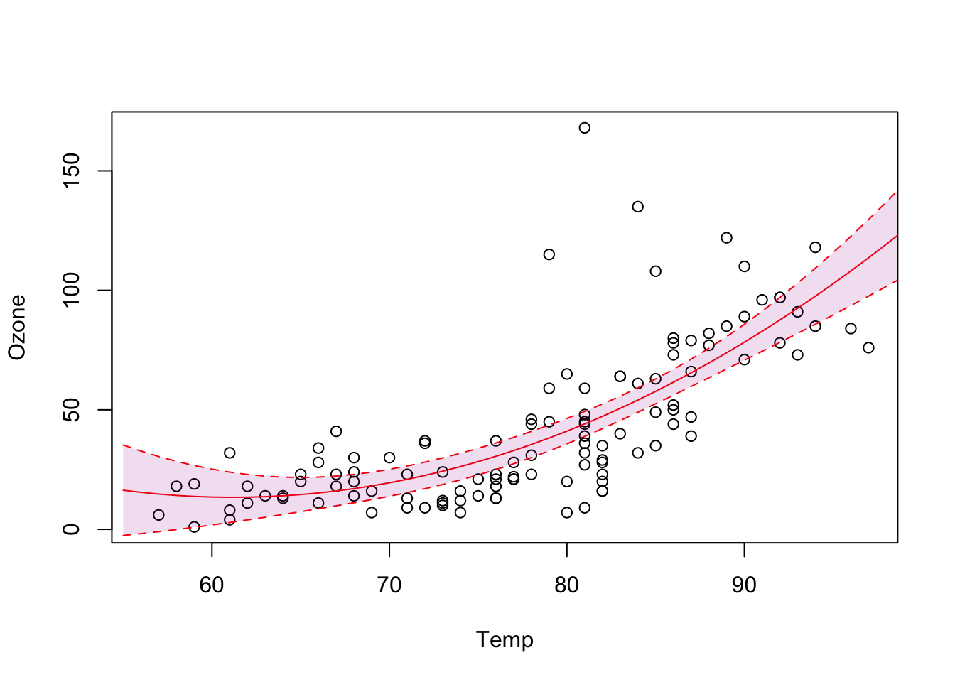
Alternative: use package effects
library(effects)
plot(effect("Temp",fit3))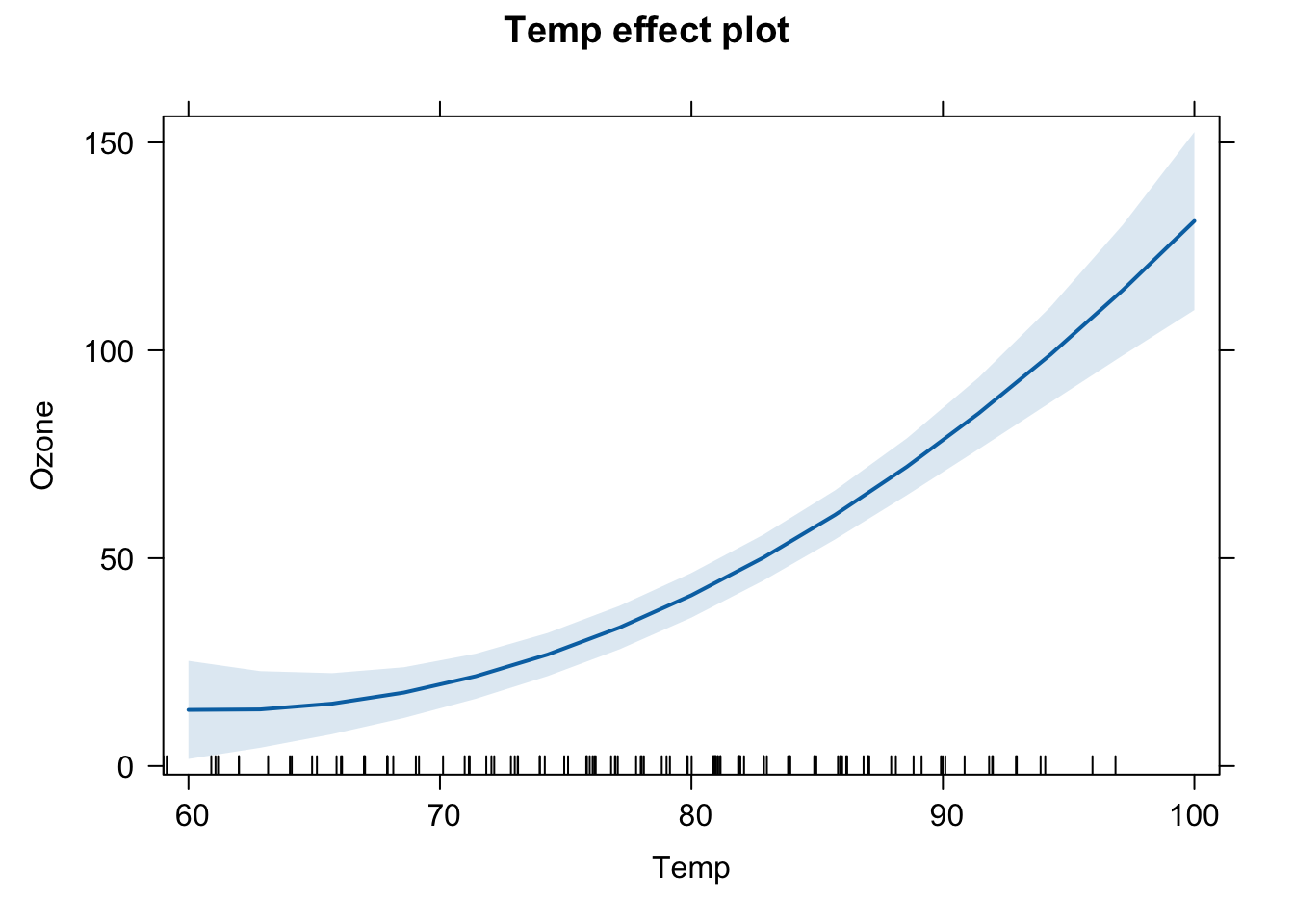
plot(effect("Temp",fit3,partial.residuals = T) ) 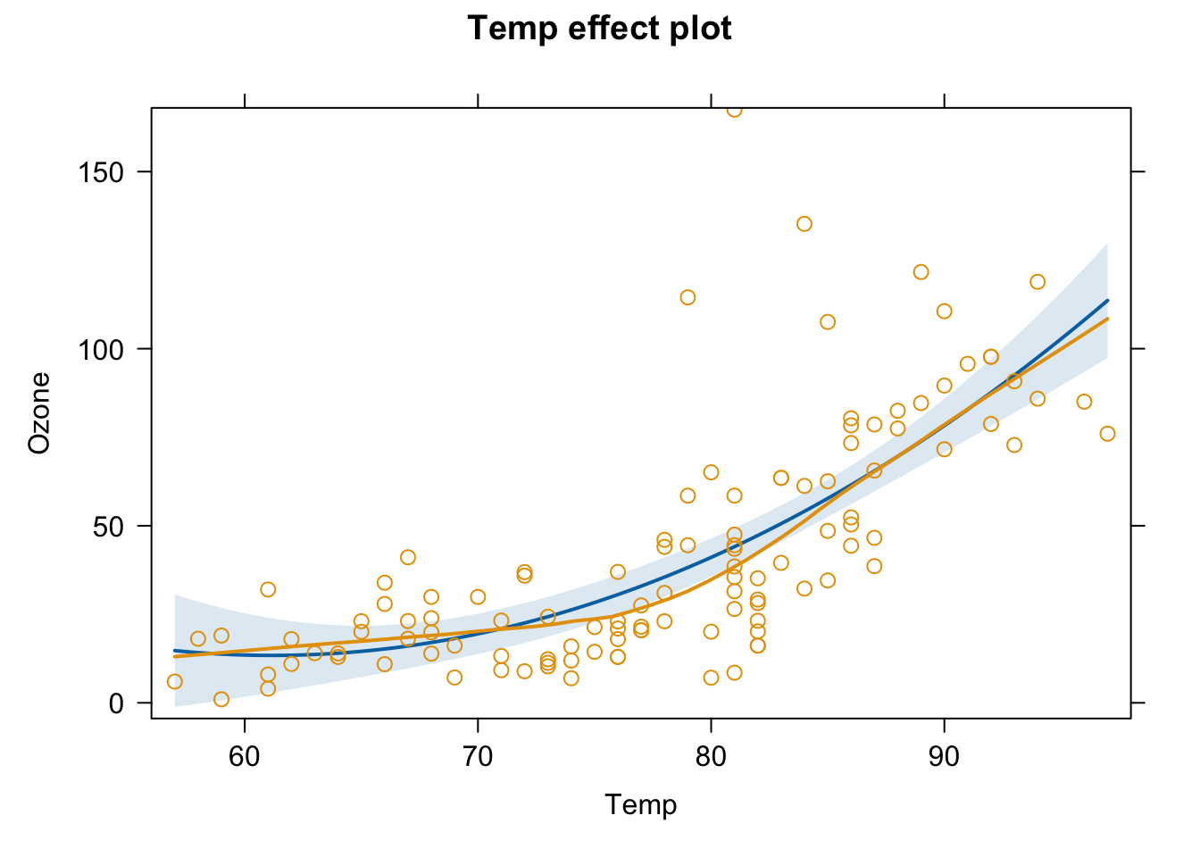
#to check patterns in residuals (plots measurements and partial residuals)Another alternative:
# or jtools package
library(jtools)
effect_plot(fit3, pred = Temp, interval = TRUE, plot.points = TRUE)