Exercise - Multiple Linear Regression

Exercise - Multiple Linear Regression

Formula syntax
Formula	Meaning	Details
`y~x_1`	\(y=a_0 +a_1*x_1\)	Slope+Intercept
`y~x_1 - 1`	\(y=a_1*x_1\)	Slope, no intercept
`y~I(x_1^2)`	\(y=a_0 + a_1*(x_1^2)\)	Quadratic effect
`y~x_1+x_2`	\(y=a_0+a_1x_1+a_2x_2\)	Multiple linear regression (two variables)
`y~x_1:x_2`	\(y=a_0+a_1(x_1x_2)\)	Interaction between x₁ and x₂
`y~x_1*x_2`	\(y=a_0+a_1(x_1x_2)+a_2x_1+a_3x_2\)	Interaction and main effects

In this exercise you will:

perform multiple linear regressions
interpret regression output and check the residuals
plot model predictions including interactions

Before you start, remember to clean your global environment (if you haven’t already) using rm(list=ls()).

To conduct the exercise, please load the following packages:

library(effects) 
## Carregando pacotes exigidos: carData
## lattice theme set by effectsTheme()
## See ?effectsTheme for details.
library(EcoData)

You will work with the following datasets:

mtcars
plantHeight form package EcoData

Useful functions

for multiple linear regression

lm() - fit linear model
summary(fit) - apply to fitted model object to display regression table
plot(fit) - plot residuals for model validation
anova(fit) - apply type I ANOVA (variables included sequentially) to model to test for effects all levels of a factor
Anova(fit) - car package; use type II ANOVA (effects for predictors when all other predictors are already included) for overall effects
scale() - scale variable
sqrt() - square-root
log() - calculates natural logarithm
plot(allEffects(fit)) - apply to fitted model object to plot marginal effect; effects package
par() - change graphical parameters
use oldpar \<- par(mfrow = c(number_rows, number_cols)) to change figure layout including more than 1 plot per figure
use par(oldpar) to reset graphic parameter

for model selection

AIC(fit) - get AIC for a fitted model
anova(fit1, fit2) - compare two fitted models via Likelihood Ratio Test (LRT)

Analyzing the `mtcars` dataset

Imagine a start up company wants to rebuild a car with a nice retro look from the 70ies. The car should be modern though, meaning the fuel consumption should be as low as possible. They’ve discovered the mtcars dataset with all the necessary measurements and they’ve somehow heard about you and your R skills and asked you for help. And of course you promised to help, kind as you are.

The company wants you to find out which of the following characteristics affects the fuel consumption measured in miles per gallon (mpg). Lower values for mpg thus reflect a higher fuel consumption. The company wants you to include the following variables into your analysis:

number of cylinders (cyl)
weight (wt)
horsepower (hp)
whether the car is driven manually or with automatic (am)

In addition, Pawl, one of the founders of the company suggested that the effect of weight (wt) might be irrelevant for powerful cars (high hp values). You are thus asked to test for this interaction in your analysis as well.

Question

Carry out the following tasks:

Perform a multiple linear regression (change class for cyl and am to factor)
Check the model residuals
Interpret and plot all effects

You may need the following functions:

as.factor()
lm()
summary()
anova()
plot()
allEffects()

Use your results to answer the questions:

Which of the following statements are correct? (Several are correct).

Cars with 6 cylinders do not differ significantly in their fuel consumption as compared to cars with 4 cylinders. Stronger cars (hp) use less fuel (mpg). Overall, heavier cars (wt) use significantly more fuel (their range is smaller; mpg)

Concerning the interaction between weight (wt) and horsepower (hp), which of the following statements is correct?

Pawl was wrong. There is a significant interaction between weight and horsepower, but the direction is opposite to what Pawl thought: The effect of weight is stronger for stronger cars. Pawl was wrong, the effect of weight is independent of horsepower. Pawl was right. The effect of weight is strong for weaker cars, but becomes indeed irrelevant for stronger cars.

This is the code that you need to interpret the results.

# change am and cyl from numeric to factor
mtcars$am <- as.factor(mtcars$am)
mtcars$cyl <- as.factor(mtcars$cyl)

# multiple linear regression and results:
# (we need to scale (standardize) the predictors wt and hp, since we include their interaction)
carsfit <- lm(mpg ~ am + cyl + scale(wt) * scale(hp), dat = mtcars)
# weight is included as the first predictor in order to have
# it as the grouping factor in the allEffects plot

summary(carsfit)
## 
## Call:
## lm(formula = mpg ~ am + cyl + scale(wt) * scale(hp), data = mtcars)
## 
## Residuals:
##     Min      1Q  Median      3Q     Max 
## -3.4121 -1.6789 -0.4446  1.3752  4.4338 
## 
## Coefficients:
##                     Estimate Std. Error t value Pr(>|t|)    
## (Intercept)          19.9064     1.5362  12.958 1.36e-12 ***
## am1                   0.1898     1.4909   0.127 0.899740    
## cyl6                 -1.2818     1.5291  -0.838 0.409813    
## cyl8                 -1.3942     2.1563  -0.647 0.523803    
## scale(wt)            -3.6248     0.9665  -3.750 0.000938 ***
## scale(hp)            -1.8602     0.8881  -2.095 0.046503 *  
## scale(wt):scale(hp)   1.5631     0.7027   2.224 0.035383 *  
## ---
## Signif. codes:  0 '***' 0.001 '**' 0.01 '*' 0.05 '.' 0.1 ' ' 1
## 
## Residual standard error: 2.246 on 25 degrees of freedom
## Multiple R-squared:  0.888,  Adjusted R-squared:  0.8612 
## F-statistic: 33.05 on 6 and 25 DF,  p-value: 1.021e-10
# The first level of each factor is used as a reference, i.e. in this case a manual gear shift with 4 gears.
# From the coefficient cyl6 we see that there is no significant difference in fuel consumption (= our response) between 4 gears (the reference) and 6 gears.
# In contrast, the predictors weight (wt) and horsepower (hp) have a significant negative effect on the range (mpg), so that they both increase fuel consumption.

# check residuals
old.par = par(mfrow = c(2, 2))
plot(carsfit)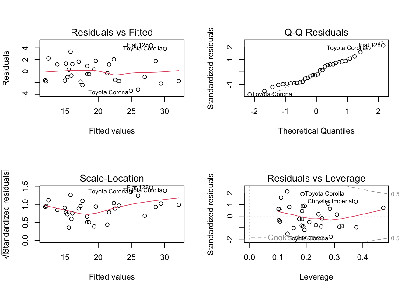

par(old.par)

# plot effects
plot(allEffects(carsfit))
## Warning in Analyze.model(focal.predictors, mod, xlevels, default.levels, : the
## predictors scale(wt), scale(hp) are one-column matrices that were converted to
## vectors
## Warning in Analyze.model(focal.predictors, mod, xlevels, default.levels, : the
## predictors scale(wt), scale(hp) are one-column matrices that were converted to
## vectors
## Warning in Analyze.model(focal.predictors, mod, xlevels, default.levels, : the
## predictors scale(wt), scale(hp) are one-column matrices that were converted to
## vectors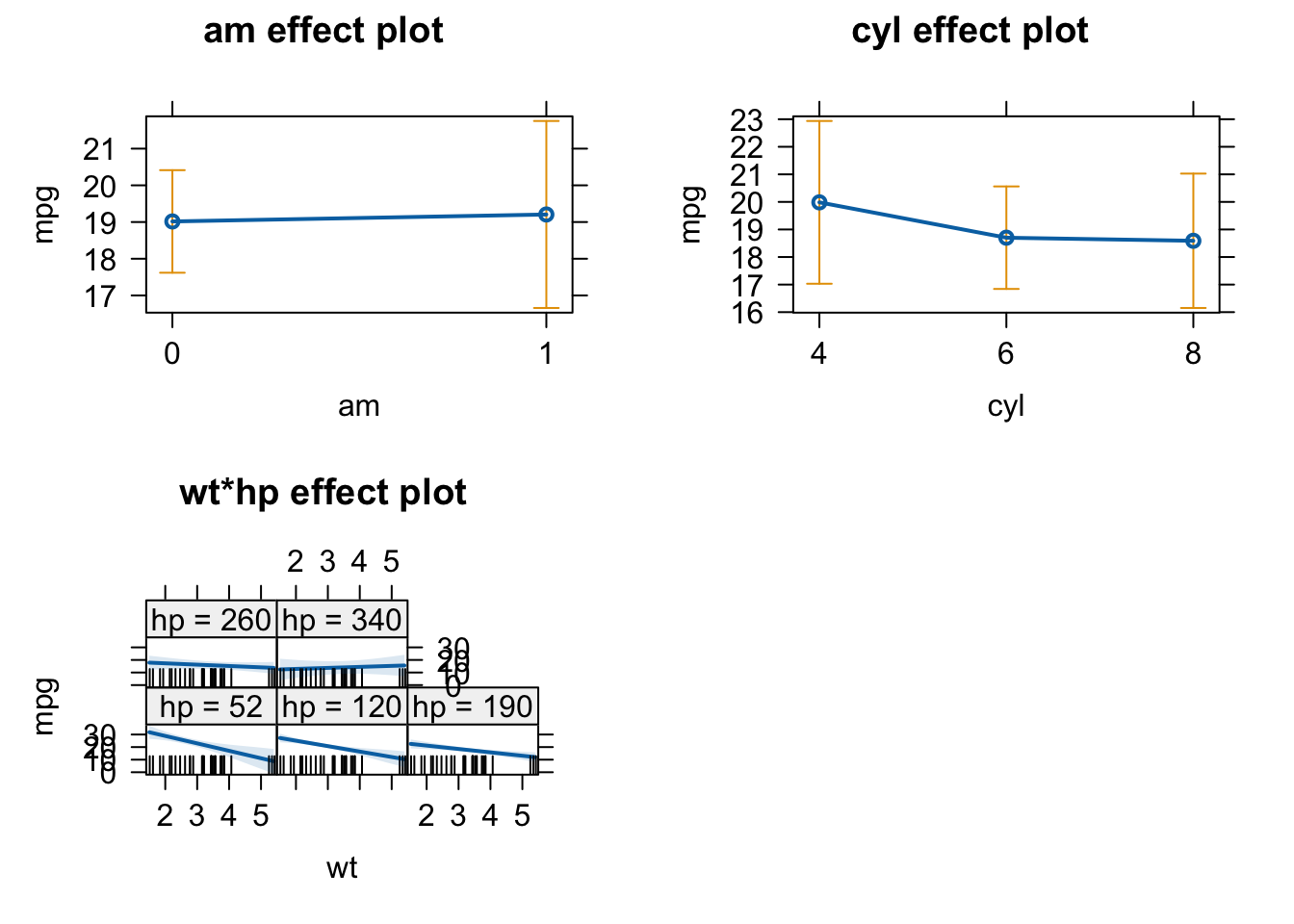

# We can see in the wt*hp plot, that for high values of hp wt has no effect on the response mpg. We conclude that Pawl was right.

Question

What is the meaning of “An effect is not significant”?
Is an effect with three *** more significant / certain than an effect with one *?

You should NOT say that the effect is zero, or that the null hypothesis has been accepted. Official language is “there is no significant evidence for an effect(p = XXX)”. If we would like to assess what that means, some people do a post-hoc power analysis (which effect size could have been estimated), but better is typically just to discuss the confidence interval, i.e. look at the confidence interval and say: if there is an effect, we are relatively certain that it is smaller than X, given the confidence interval of XYZ.
Many people view it that way, and some even write “highly significant” for *** . It is probably true that we should have a slightly higher confidence in a very small p-value, but strictly speaking, however, there is only significant, or not significant. Interpreting the p-value as a measure of certainty is a slight misinterpretation. Again, if we want to say how certain we are about the effect, it is better to look again at the confidence interval, i.e. the standard error and use this to discuss the precision of the estimate (small confidence interval / standard error = high precision / certainty).

Interactions with the `plantHeight` dataset

Plant Height

Use the plantHeight dataset from EcoData package.

library(EcoData)
#str(plantHeight)

Model (separate) multiple regressions form log of height (loght) to test if:

If temp (temperature) or NPP (net primary productivity) is a more important predictor (importance == scaled effect size).
If growth forms (variable growthform) differ in their temperature (temp) effects. (use an interaction AND relevel your factor variable to have the Herb growth form in the intercept - see the function relevel)
If the effect of temp remains significant if we include latitude (lat) and an interaction of latitude with temp. If not, why? Tip: plot temp ~ lat.

plantHeight$sTemp = scale(plantHeight$temp)
plantHeight$sLat = scale(plantHeight$lat)
plantHeight$sNPP = scale(plantHeight$NPP)

# relevel 
plantHeight$growthform2 = relevel(as.factor(plantHeight$growthform), "Herb")

NPP or Temp?

fit = lm(loght ~ sTemp + sNPP, data = plantHeight)
summary(fit)
## 
## Call:
## lm(formula = loght ~ sTemp + sNPP, data = plantHeight)
## 
## Residuals:
##      Min       1Q   Median       3Q      Max 
## -1.69726 -0.47935  0.04285  0.39812  1.77919 
## 
## Coefficients:
##             Estimate Std. Error t value Pr(>|t|)    
## (Intercept)  0.44692    0.05119   8.731 2.36e-15 ***
## sTemp        0.20846    0.07170   2.907 0.004134 ** 
## sNPP         0.24734    0.07164   3.452 0.000702 ***
## ---
## Signif. codes:  0 '***' 0.001 '**' 0.01 '*' 0.05 '.' 0.1 ' ' 1
## 
## Residual standard error: 0.6711 on 169 degrees of freedom
##   (6 observations deleted due to missingness)
## Multiple R-squared:  0.2839, Adjusted R-squared:  0.2754 
## F-statistic:  33.5 on 2 and 169 DF,  p-value: 5.553e-13

NPP is slightly more important.

Interaction with growth form

fit = lm(loght ~ growthform2 *  sTemp , data = plantHeight)
summary(fit)
## 
## Call:
## lm(formula = loght ~ growthform2 * sTemp, data = plantHeight)
## 
## Residuals:
##      Min       1Q   Median       3Q      Max 
## -1.19634 -0.21217 -0.00997  0.22750  1.62398 
## 
## Coefficients: (2 not defined because of singularities)
##                              Estimate Std. Error t value Pr(>|t|)    
## (Intercept)                 -0.310748   0.062150  -5.000 1.51e-06 ***
## growthform2Fern              0.624160   0.375650   1.662 0.098586 .  
## growthform2Herb/Shrub        0.456394   0.377088   1.210 0.227967    
## growthform2Shrub             0.562799   0.083100   6.773 2.36e-10 ***
## growthform2Shrub/Tree        0.957088   0.486858   1.966 0.051069 .  
## growthform2Tree              1.586005   0.080756  19.640  < 2e-16 ***
## sTemp                        0.203808   0.053231   3.829 0.000185 ***
## growthform2Fern:sTemp              NA         NA      NA       NA    
## growthform2Herb/Shrub:sTemp        NA         NA      NA       NA    
## growthform2Shrub:sTemp       0.103357   0.076860   1.345 0.180636    
## growthform2Shrub/Tree:sTemp -0.004614   0.526866  -0.009 0.993024    
## growthform2Tree:sTemp       -0.244410   0.077661  -3.147 0.001971 ** 
## ---
## Signif. codes:  0 '***' 0.001 '**' 0.01 '*' 0.05 '.' 0.1 ' ' 1
## 
## Residual standard error: 0.3713 on 158 degrees of freedom
##   (10 observations deleted due to missingness)
## Multiple R-squared:  0.796,  Adjusted R-squared:  0.7844 
## F-statistic: 68.51 on 9 and 158 DF,  p-value: < 2.2e-16

Yes, because (some) interactions are significant.

Note that the n.s. effect of sTemp is the first growth form (Ferns), for which we had only one observation. In a standard multiple regression, you don’t have p-values for the significance of the temperature effect against 0 for the other growth forms, because you test against the reference. What one usually does is to run an ANOVA to see if temp is overall significant.

anova(fit)
## Analysis of Variance Table
## 
## Response: loght
##                    Df Sum Sq Mean Sq  F value    Pr(>F)    
## growthform2         5 78.654 15.7309 114.1241 < 2.2e-16 ***
## sTemp               1  3.543  3.5426  25.7006 1.104e-06 ***
## growthform2:sTemp   3  2.800  0.9333   6.7707 0.0002524 ***
## Residuals         158 21.779  0.1378                       
## ---
## Signif. codes:  0 '***' 0.001 '**' 0.01 '*' 0.05 '.' 0.1 ' ' 1

Alternatively, if you want to test if a specific growth form has a significant temperature effect, you could either extract the p-value from a multiple regression (a bit complicated) or just run a univariate regression for this growth form

fit = lm(loght ~ sTemp + 0, data = plantHeight[plantHeight$growthform == "Tree",])
summary(fit)
## 
## Call:
## lm(formula = loght ~ sTemp + 0, data = plantHeight[plantHeight$growthform == 
##     "Tree", ])
## 
## Residuals:
##    Min     1Q Median     3Q    Max 
## 0.2636 0.7198 0.9672 1.3503 2.3914 
## 
## Coefficients:
##       Estimate Std. Error t value Pr(>|t|)   
## sTemp   0.5013     0.1699    2.95  0.00452 **
## ---
## Signif. codes:  0 '***' 0.001 '**' 0.01 '*' 0.05 '.' 0.1 ' ' 1
## 
## Residual standard error: 1.21 on 60 degrees of freedom
##   (10 observations deleted due to missingness)
## Multiple R-squared:  0.1267, Adjusted R-squared:  0.1121 
## F-statistic: 8.704 on 1 and 60 DF,  p-value: 0.004522

Or you could fit the interaction but turn-off the intercept (by saying +0 or -1) and remove the plantHeight intercepts:

fit = lm(loght ~ sTemp:growthform + 0, data = plantHeight)
summary(fit)
## 
## Call:
## lm(formula = loght ~ sTemp:growthform + 0, data = plantHeight)
## 
## Residuals:
##     Min      1Q  Median      3Q     Max 
## -1.5156 -0.1396  0.3488  0.8103  2.3914 
## 
## Coefficients:
##                            Estimate Std. Error t value Pr(>|t|)    
## sTemp:growthformFern        -0.8949     2.9233  -0.306 0.759911    
## sTemp:growthformHerb         0.3195     0.1077   2.967 0.003460 ** 
## sTemp:growthformHerb/Shrub   1.1788     5.5825   0.211 0.833026    
## sTemp:growthformShrub        0.2375     0.1197   1.984 0.048974 *  
## sTemp:growthformShrub/Tree   0.8833     0.2613   3.380 0.000908 ***
## sTemp:growthformTree         0.5013     0.1171   4.281 3.17e-05 ***
## ---
## Signif. codes:  0 '***' 0.001 '**' 0.01 '*' 0.05 '.' 0.1 ' ' 1
## 
## Residual standard error: 0.8339 on 162 degrees of freedom
##   (10 observations deleted due to missingness)
## Multiple R-squared:  0.2083, Adjusted R-squared:  0.179 
## F-statistic: 7.106 on 6 and 162 DF,  p-value: 9.796e-07

Interaction with lat

fit = lm(loght ~ sTemp * sLat, data = plantHeight)
summary(fit)
## 
## Call:
## lm(formula = loght ~ sTemp * sLat, data = plantHeight)
## 
## Residuals:
##      Min       1Q   Median       3Q      Max 
## -1.97905 -0.45112  0.01062  0.42852  1.74054 
## 
## Coefficients:
##             Estimate Std. Error t value Pr(>|t|)    
## (Intercept)  0.46939    0.06771   6.932 7.78e-11 ***
## sTemp        0.26120    0.14200   1.839   0.0676 .  
## sLat        -0.13072    0.13616  -0.960   0.3383    
## sTemp:sLat   0.01209    0.04782   0.253   0.8007    
## ---
## Signif. codes:  0 '***' 0.001 '**' 0.01 '*' 0.05 '.' 0.1 ' ' 1
## 
## Residual standard error: 0.6869 on 174 degrees of freedom
## Multiple R-squared:  0.2504, Adjusted R-squared:  0.2375 
## F-statistic: 19.37 on 3 and 174 DF,  p-value: 6.95e-11

All is n.s. … how did this happen? If we check the correlation between temp and lat, we see that the two predictors are highly collinear.

cor(plantHeight$temp, plantHeight$lat)
## [1] -0.9249304

In principle, the regression model should be able to still separate them, but the higher the collinearity, the more difficult it becomes for the regression to infer if the effect is caused by one or the other predictor.

Model selection with the Plant Height data

Plant Height

Use the plantHeight data and the previously fitted models to loght.

Compare nested models built with the variables Temp and growthform through anova().

Compare all models fitted before with AIC.

What’s your conclusion?

Building models with Temp and growthform. But first, excluding rows with NA in any of these variables (loght as well) - you can’t compare models with different number of data points!!

plantNew <- plantHeight[, c("loght", "growthform2", "sTemp")]
plantNew <- na.omit(plantNew)

fit1 = lm(loght ~ growthform2, data = plantNew)
fit2 = lm(loght ~ sTemp, data = plantNew)
fit3 = lm(loght ~ growthform2 + sTemp, data = plantNew)
fit4 = lm(loght ~ growthform2*sTemp, data = plantNew)

Comparing nested models with anova:

anova(fit1,fit3,fit4)
## Analysis of Variance Table
## 
## Model 1: loght ~ growthform2
## Model 2: loght ~ growthform2 + sTemp
## Model 3: loght ~ growthform2 * sTemp
##   Res.Df    RSS Df Sum of Sq       F    Pr(>F)    
## 1    162 28.121                                   
## 2    161 24.578  1    3.5426 25.7006 1.104e-06 ***
## 3    158 21.779  3    2.7998  6.7707 0.0002524 ***
## ---
## Signif. codes:  0 '***' 0.001 '**' 0.01 '*' 0.05 '.' 0.1 ' ' 1
anova(fit2,fit3,fit4)
## Analysis of Variance Table
## 
## Model 1: loght ~ sTemp
## Model 2: loght ~ growthform2 + sTemp
## Model 3: loght ~ growthform2 * sTemp
##   Res.Df    RSS Df Sum of Sq       F    Pr(>F)    
## 1    166 80.526                                   
## 2    161 24.579  5    55.947 81.1767 < 2.2e-16 ***
## 3    158 21.779  3     2.800  6.7707 0.0002524 ***
## ---
## Signif. codes:  0 '***' 0.001 '**' 0.01 '*' 0.05 '.' 0.1 ' ' 1
anova(fit3,fit4)
## Analysis of Variance Table
## 
## Model 1: loght ~ growthform2 + sTemp
## Model 2: loght ~ growthform2 * sTemp
##   Res.Df    RSS Df Sum of Sq      F    Pr(>F)    
## 1    161 24.578                                  
## 2    158 21.779  3    2.7998 6.7707 0.0002524 ***
## ---
## Signif. codes:  0 '***' 0.001 '**' 0.01 '*' 0.05 '.' 0.1 ' ' 1

Comparing all models with AIC

res <- AIC(fit1,fit2,fit3,fit4)
res <- res[order(res$AIC),] # ordering lowest AIC
res$deltaAIC <- res$AIC - res$AIC[1] # including deltaAIC
res
##      df      AIC  deltaAIC
## fit4 11 155.5342   0.00000
## fit3  8 169.8521  14.31792
## fit1  7 190.4728  34.93864
## fit2  3 359.2179 203.68365

Useful functions

Analyzing the mtcars dataset

Interactions with the plantHeight dataset

Model selection with the Plant Height data

Analyzing the `mtcars` dataset

Interactions with the `plantHeight` dataset