learn how to choose an appropriate test and interpret its result
practice these tests in R
practice the simulation of data and error rates
But before we go into these topics, however, we need to discuss how data arises, and how we represent it.
6.1 Sample, population, and the data-generating process
The very reason for doing statistics is that the data that we observe is somehow random. But how does this randomness arise?
Imagine that we are interested in the average growth rate of trees in Germany during two consecutive years. Ideally, we would measure them all and be done, without having to do statistics. In practice, however, we hardly ever have the resources to do so. We therefore have to make a selection of trees, and infer the growth rate of all trees from that. The statistical term for all the trees is the “population”, and the term for the trees that you have observed is the “sample”. Hence, we want to infer properties of the population from a sample.
The population is the set of all observations that you could have made. The sample is the observations that you have actually made.
The population as such is fixed and does not change, but every time we observe a random selection (sample) of the population, we may get elements with slightly different properties. As a concrete example: imagine we have the resources to only sample 1000 trees across Germany. Thus, every time we take a random selection of 1000 trees out of the population, we will get a slightly different average growth rate.
Sampling creates randomness.
The process of sampling from the population does explain how randomness arises in our data. However, a slight issue with this concept is that it does not match very well with more complex random processes. Imagine, for example, that data arises from a person going to randomly selected plots to measure radiation (which varies within minutes due to cloud cover), using a measurement instrument that measures with some random error. Does it really make sense to think of the data arising from sampling from a “population” of possible observations?
However, not all randomness comes from sampling from a population.
A more modern and general concept to describe how data is created is the concept of the “data-generating process”, which is pretty self-explanatory: the data-generating process describes how the observations from a random sample arise, including systematic and stochastic processes. It therefore includes the properties of what would classically be called “sampling from a population”, but it is broader and includes all other processes that would create systematic and random patterns in our data. In this picture, instead of inferring properties of the population from a sample, we would say we want to infer the properties of the data-generating process from a sample of observations created by this process.
A more modern concept that replaces the “population” is the “data-generating process”. The data-generating process describes how the observations from a random sample arise, including systematic and stochastic processes.
Whether you think in populations or data-generating processes: the important point to remember from this section is that there are two objects that we have to distinguish well: on the one hand, there is our sample. We may describe it in terms of it’s properties (mean, minimum, maximum), but the sample is not the final goal. Ultimately, we want to infer the properties of the population / data-generating process from the sample. We will explain how to do this in the next sections, in particular in the section on inferential statistics. Before we come to that, however, let us talk in a bit more detail about the representation of the sample, i.e. the data that we observe.
6.2 A recipe for hypothesis testing
Aim: We want to know if there is a difference between the control and the treatment.
We introduce a Null hypothesis H0 (e.g. no effect, no difference between control and treatment)
We invent a test statistic
We calculate the expected distribution of our test statistic given H0 (this is from our data-generating model)
We calculate the p-value = probability of getting observed test statistic or more extreme given that H0 is true (there is no effect): \(p-value = P(d\ge D_{obs} | H_0)\)
WarningInterpretation of the p-value
p-values make a statement on the probability of the data or more extreme values given H0 (no effect exists), but not on the probability of H0 (no effect) and not on the size of the effect or on the probability of an effect!
If you want to read more about null hypothesis testing and the p-value, take a look at Daniel Lakens Book
Example:
Imagine we do an experiment with two groups, one treatment and one control group. Test outcomes are binary, e.g. whether individuals are cured (1) or not (0).
We need a test statistic. For example: proportion of cured patients in the treatment group from the total number of cured patients: treat/(treat+control)
We need the distribution of this test statistic under the null hypothesis (of no diference in proportion of cured patients between .
Let’s create a true world without effect:
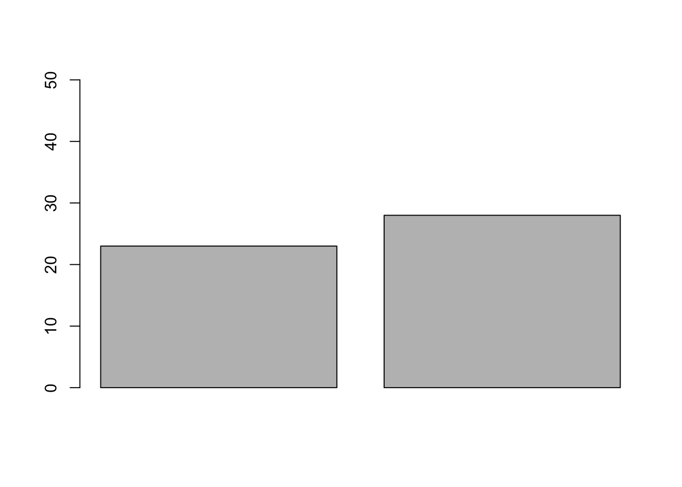
set.seed(123)PperGroup =50# number of replicates (e.g., persons per treatment group)pC =0.5#probability of being cured in control grouppT =0.5#probability of being cured in treatment group;# pT is the same as pC, because we want to use these to get the distribution of the test statistic we define below when H0 is true (no effect)# Let's draw a sample from this world without effectcontrol =rbinom(n =1, size = PperGroup, prob = pC)treat =rbinom(n =1, size = PperGroup, prob = pT)# calculate the test statistic: treat/(treat+control)## [1] 0.5490196# and plotbarplot(c(control, treat), ylim =c(0, 50), names.arg =c("control", "treatment"),ylab ="Counts (cured patients)",main="Number of cured patients out of 50")
why do whe use set.seed() here? Read the help file of the function to understand it! help(set.seed). Experiment changing the number in the set seed in your code and compare the results for tne number of cured patients in the treatment and control groups.
The table with the results of the experiment would be:
data <-data.frame(treatment =rep(c("control", "treatment"), each =50),cured =c(rep(c(0,1), times=c(50-control, control)),rep(c(0,1), times=c(50-treat, treat))))table(data$treatment, data$cured)## ## 0 1## control 27 23## treatment 22 28
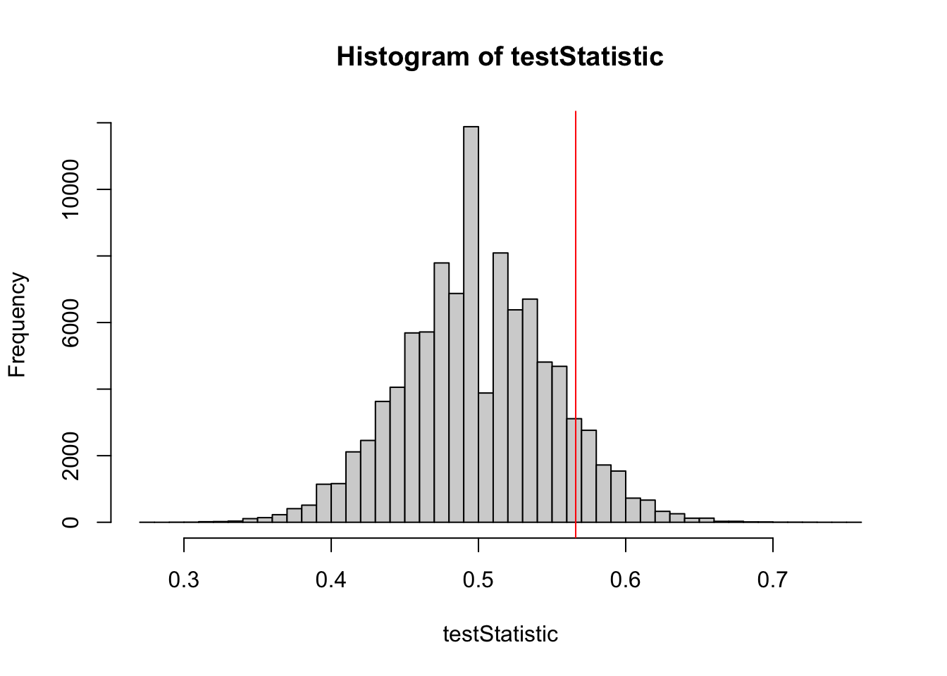
Now, let’s do this very often (100,000 times!) to get the distribution under H0 (generating a null distribution of proportion of cured patients in the treatment group):
testStatistic =rep(NA, 100000) # to store our resultsfor (i in1:100000) { control =rbinom(n =1, size = PperGroup, prob = pC) treat =rbinom(n =1, size = PperGroup, prob = pT) testStatistic[i] = treat/(treat+control) # test statistic }hist(testStatistic, breaks =50)
If you are confused with the for loop, read about it here
We now have our test statistic + the frequency distribution of our statistic if the H0 is true. Now we make an experiment: Assume that we observed the data we simulated first (our barplot): Control = 23, Treatment = 28.
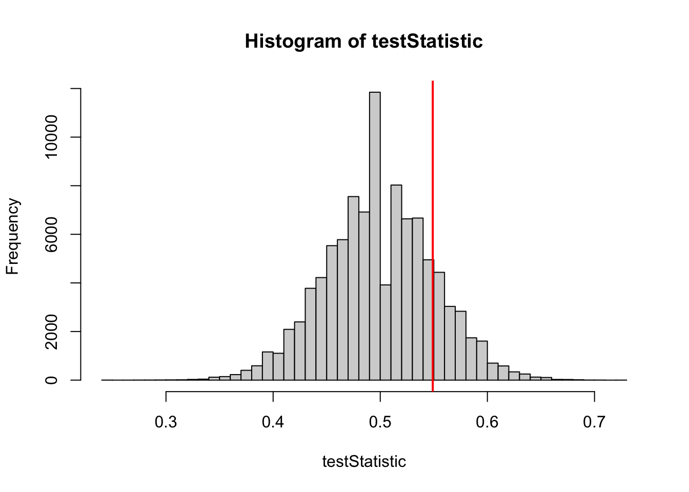
hist(testStatistic, breaks =50)testStatisticData =28/(28+23)abline(v = testStatisticData, col ="red", lwd =2)
mean(testStatistic > testStatisticData)## [1] 0.16044# compare each value in our testStatistic distribution with# the observed value and calculate proportion of TRUE values # (where testStatistic > testStatisticData)
But we know actually that the test statistic follows a Chi2 distribution. So to get correct p-values we can use the prop.test for this test statistic:
prop.test(c(28, 23), c(PperGroup, PperGroup))## ## 2-sample test for equality of proportions with continuity correction## ## data: c(28, 23) out of c(PperGroup, PperGroup)## X-squared = 0.64026, df = 1, p-value = 0.4236## alternative hypothesis: two.sided## 95 percent confidence interval:## -0.1149746 0.3149746## sample estimates:## prop 1 prop 2 ## 0.56 0.46# other test statistic with known distribution# Pearson's chi-squared test statistic# no need to simulate
We pass the data to the function which first calculates the test statistic and then calculates the p-value using the Chi2 distribution.
6.3 t-test
Originally developed by Wiliam Sealy Gosset (1876-1937) who has worked in the Guinness brewery. He wanted to measure which ingredients result in a better beer. The aim was to compare two beer recipes and decide whether one of the recipes was better (e.g. to test if it results in more alcohol). He published under the pseudonym ‘Student’ because the company considered his statistical methods as a commercial secret.
Importantt-test assumptions
Data in both groups is normally distributed
H0 : the means of both groups are equal
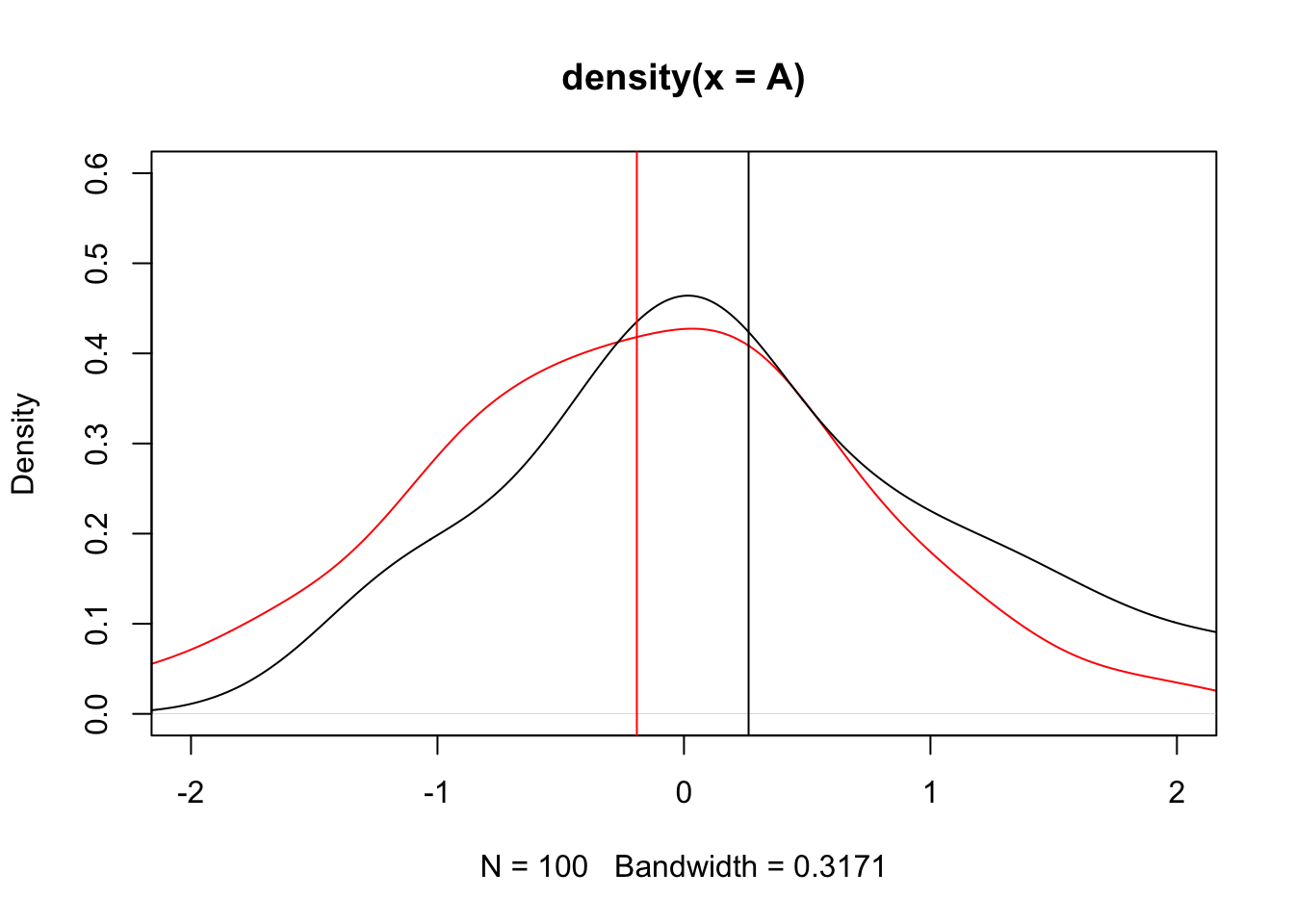
The idea is that we have two normal distributions (e.g. alcohol distributions) to compare means. Let’s simulate some data and see the distribution of both groups:
Code
set.seed(1)A =rnorm(100, mean =-.3)B =rnorm(100, mean = .3)plot(density(A), col ="red", xlim =c(-2, 2), ylim =c(0, 0.6))lines(density(B))abline(v =mean(A), col ="red")text(x =mean(A)-0.4, y =0.5, labels ="Mean A", pos =3, xpd =NA, col ="red")abline(v =mean(B))text(x =mean(B)+0.4, y =0.5, labels ="Mean B", pos =3, xpd =NA, col ="black")
And our goals is now to test if the difference between the two means of the variables is statistically significant or not.
Procedure:
Calculate variances and means of both variables
A_m =mean(A)B_m =mean(B)A_v =var(A)B_v =var(B)
Calculate t-statistic (difference between means / (Standard deviations/sample sizes)): \(t = \frac{\bar{x}_1 - \bar{x}_2}{\sqrt{\frac{s_1^2}{n_1} + \frac{s_2^2}{n_2}}}\)
Compare observed t with t distribution under H0 (which we can do by using the CDF function of the t-distribution:
pt( t_statistic, # test statisticdf =length(A)+length(B)-2, # degrees of freedom, roughly = n_obs - n_parameterslower.tail =TRUE )*2## [1] 0.0006799933
CautionOne-sided or two-sided
If we do NOT know if the dataset from one group is larger or smaller than the other, we must use two-sided tests (that’s why we multiply the p-values with 2). Only if we are sure that the effect MUST be positive / negative, we can test for greater / less. Decide BEFORE you look at the data!
Let’s compare it to the output of the t.test function which does everything for us, we only need to pass the data to the function:
t.test(A, B, var.equal =TRUE)## ## Two Sample t-test## ## data: A and B## t = -3.4521, df = 198, p-value = 0.00068## alternative hypothesis: true difference in means is not equal to 0## 95 percent confidence interval:## -0.7122549 -0.1943542## sample estimates:## mean of x mean of y ## -0.1911126 0.2621919
Usually we also have to test for normality of our data, which we can do with another test, for example the Shapiro-Wilk test:
# attention: t test assumes normal dirstribution of measurements in both groups!shapiro.test(A)## ## Shapiro-Wilk normality test## ## data: A## W = 0.9956, p-value = 0.9876shapiro.test(B)## ## Shapiro-Wilk normality test## ## data: B## W = 0.97431, p-value = 0.04763
Because we know our data comes from a normal distribution (we simulated from there), the example above is boring. Let’s have a look on the normality test with real data:
# let's use only two groups control and treatment1:ctrl = PlantGrowth$weight[PlantGrowth$group =="ctrl"]trt1 = PlantGrowth$weight[PlantGrowth$group =="trt1"]# test normality before doing the t test:shapiro.test(ctrl)## ## Shapiro-Wilk normality test## ## data: ctrl## W = 0.95668, p-value = 0.7475shapiro.test(trt1)## ## Shapiro-Wilk normality test## ## data: trt1## W = 0.93041, p-value = 0.4519t.test(ctrl, trt1)## ## Welch Two Sample t-test## ## data: ctrl and trt1## t = 1.1913, df = 16.524, p-value = 0.2504## alternative hypothesis: true difference in means is not equal to 0## 95 percent confidence interval:## -0.2875162 1.0295162## sample estimates:## mean of x mean of y ## 5.032 4.661# note that this is a "Welch" t-test# we will have a look at the differences among t-tests in the next large exercise
From the example above, comparing weight of two groups, answer the questions:
What is H0?
What is the result?
Explain the different values in the output!
WarningShapiro - Test for normality
If you have a small sample size, the shapiro test will always be non-significant (i.e. not significantly different from a normal distribution)! This is because small sample size leads to low power for rejecting H0 of normal distribution. You will see about power in the end of this chapter.
6.4 Type I error rate
Let’s start with a small simulation example of comparing two means with t-test. Simulating many times from a world without effect:
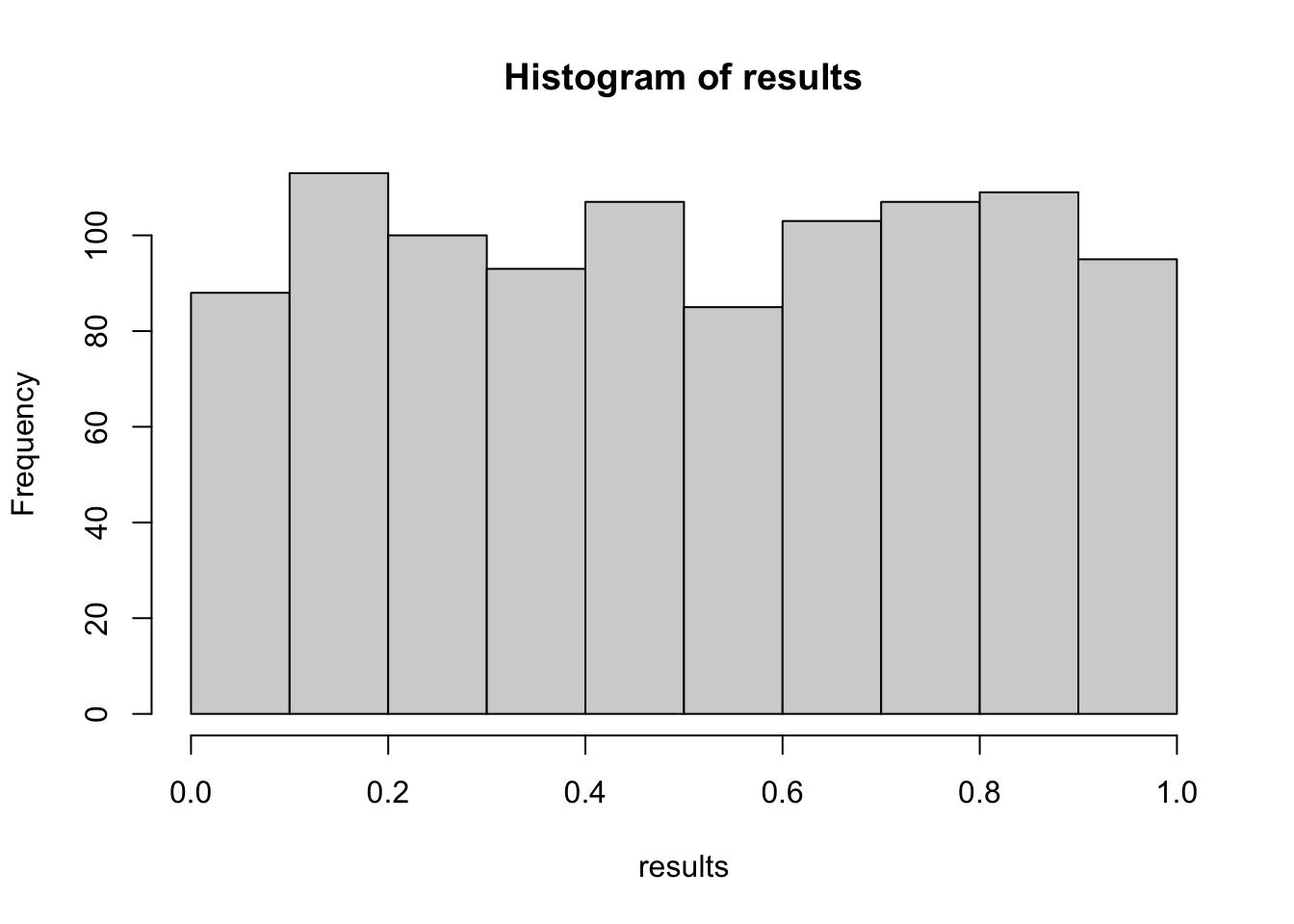
results =replicate(1000, { A =rnorm(100, mean =0.0) B =rnorm(100, mean =0.0)t.test(A, B)$p.value})hist(results)
What’s happening here? We have no effect in our simulation but there are many p-values lower than \(\alpha = 0.05\):
mean(results <0.05)## [1] 0.043
So in 4.3 % of our experiments we would reject H0 even when there is no effect at all! This is called the type I error rate. Those are false positives.
6.4.1 Type I error rate and multiple testing
If there is no effect, the probability of having a positive test result is equal to the significance level \(\alpha\). If you test 20 things that don’t have an effect, you will have one significant result on average when using a significance level of 0.05. If multiple tests are done, a correction for multiple testing should be used.
This problem is called multiple testing:
e.g.: if you try 20 different analyses (Null hypotheses), on average one of them will be significant.
e.g.: if you test 1000 different genes for their association with cancer, and in reality, none of them is related to cancer, 50 out of the tests will still be significant even if there is no effect.
If multiple tests are done, a correction for multiple testing should be used.
To increase the p-values for each test in a way that the overall alpha level is 0.05:
Let’s see it with the plantGrowth data:
# conduct a t-test for each of the treatment combinations# save each test as a new object (test 1 to 3)control = PlantGrowth$weight[PlantGrowth$group =="ctrl"]trt1 = PlantGrowth$weight[PlantGrowth$group =="trt1"]trt2 = PlantGrowth$weight[PlantGrowth$group =="trt2"]test1 =t.test(control, trt1)test2 =t.test(control, trt2)test3 =t.test(trt1, trt2)# the 3 p-valuesc(test1$p.value, test2$p.value, test3$p.value)## [1] 0.250382509 0.047899256 0.009298405
We see that two of the three tests are significant at the \(\alpha\)=0.05 level. But we have to adjust this to avoid false positives. One example is using the p.adjust function. This function has 3 methods:
p.adjust(c(test1$p.value, test2$p.value, test3$p.value)) # standard is holm, average conservative## [1] 0.25038251 0.09579851 0.02789521p.adjust(c(test1$p.value, test2$p.value, test3$p.value), method ="bonferroni") # conservative## [1] 0.75114753 0.14369777 0.02789521p.adjust(c(test1$p.value, test2$p.value, test3$p.value), method ="BH") # least conservative## [1] 0.25038251 0.07184888 0.02789521# for details on the methods see help of ?p.adjust
We end up with only one significant t-test after adjusting for multiple testing, the one comparing treatment 1 and 2.
If multiple testing is a problem and if we want to avoid false positives (type I errors), why don’t we use a smaller alpha level? Because if would increase the type II error rate.
6.5 Type II error rate
It can also happen the other way around:
results =replicate(1000, { A =rnorm(100, mean =0.0) B =rnorm(100, mean =0.2) # effect is there!t.test(A, B)$p.value})hist(results)
mean(results <0.05)## [1] 0.292
Now, we wouldn’t reject the H0 in 70.8% of our experiments. This is the type II error rate (false negatives).
The type II error rate (\(\beta\)) is affected by:
After the experiment, the only parameter we could change would be the significance level \(\alpha\), but increasing it would result in too high Type I error rates.
6.6 Statistical power
We can reduce \(\alpha\) and we will get fewer type I errors (false positives), but type II errors (false negatives) will increase. So what can we do with this in practice?
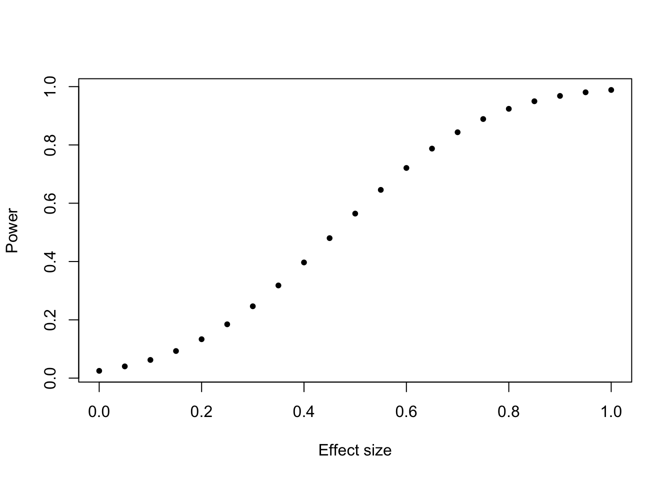
1- \(\beta\) is the so called statistical power which is the rate at which a test is significant if the effect truly exists. Power increases with stronger effect, smaller variability, (larger \(\alpha\) ), and more data (sample size). So, collect more data? How much data do we need?
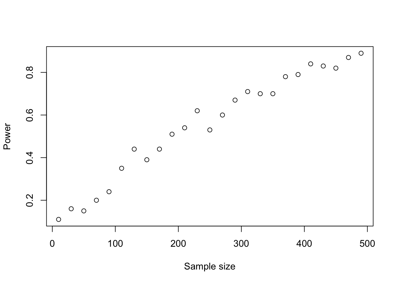
Before the experiment, you can guess the effect size and the variability, and together with alpha (known), you can calculate the power depending on the sample size:
Code
results =sapply(seq(10, 500, by =20), function(n) { results =replicate(100, { A =rnorm(n, mean =0.0) B =rnorm(n, mean =0.2) # effect is theret.test(A, B)$p.value }) power =1-mean(results >0.05)return(power) })plot(seq(10, 500, by =20), results, xlab ="Sample size", ylab ="Power", main ="")
We call that a power analysis and there’s a function in R to do that:
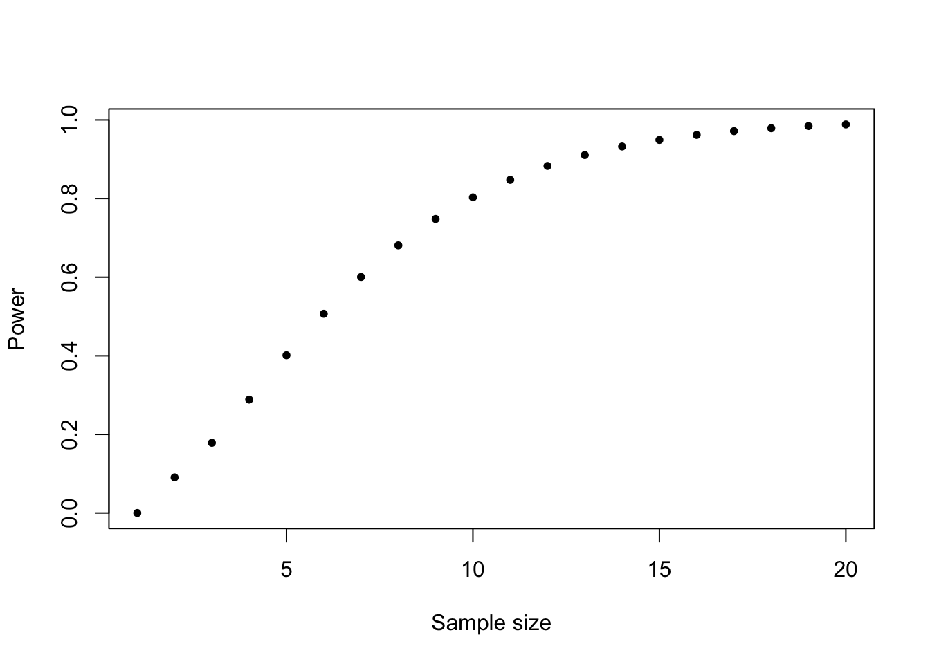
power.t.test(n =10, delta =1, sd =1, type ="one.sample")## ## One-sample t test power calculation ## ## n = 10## delta = 1## sd = 1## sig.level = 0.05## power = 0.8030962## alternative = two.sided
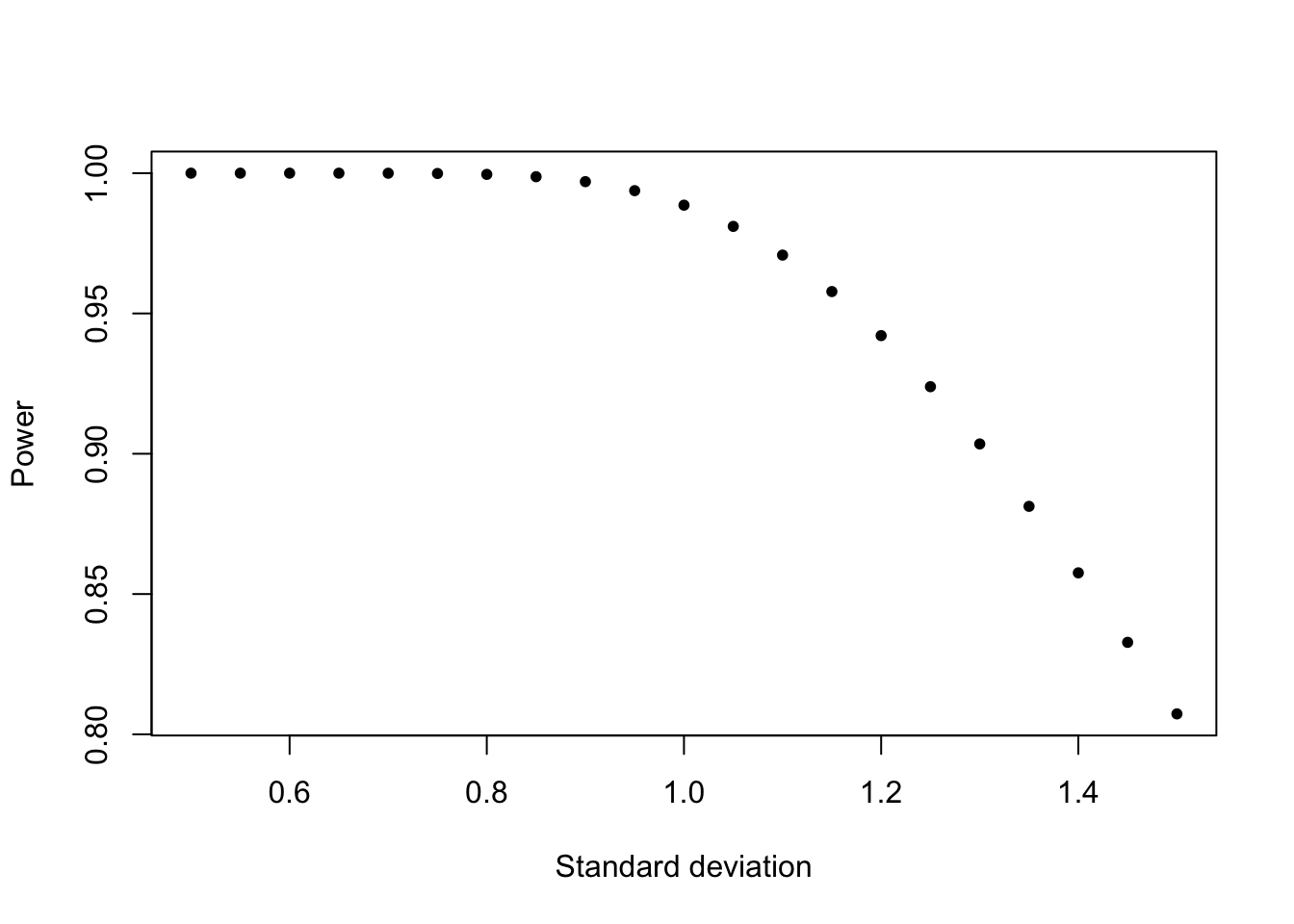
Power increases with sample size (effect size constant, sd constant):
You may have realized that if we do an experiment with a (weak) effect, we can get a significant result because of the effect but also significant results because of the Type I error rate. How to distinguish between those two? How can we decide whether a significant result is a false positive? This error rate is called the false discovery rate and to lower it we need to increase the power:
\(p(H_0)\) = probability of H0 (no effect); \(p(!H_0)\) = probability of not H0 (effect exists). Both are unknown and the only parameters we can influence are \(\alpha\) and \(\beta\). But decreasing \(\alpha\) leads to too high false negatives, so \(\beta\) is left.