[[10]{.chapter-number}  [Generalized linear models]{.chapter-title}]{#sec-glm .quarto-section-identifier}

10 Generalized linear models

We will start by fiting a linear regression (not yet a GLM) to the titanic survival dataset (in EcoData package. Let’s model the survival as a linear combination of age and sex:

library(EcoData) # titanic data

#str(titanic) #from EcoData package
#Convert pclass (passenger class) to a factor for modeling
titanic$Fpclass = as.factor(titanic$pclass)

m = lm(survived~age+sex, data = titanic)
summary(m)
## 
## Call:
## lm(formula = survived ~ age + sex, data = titanic)
## 
## Residuals:
##     Min      1Q  Median      3Q     Max 
## -0.7728 -0.2100 -0.1954  0.2484  0.8308 
## 
## Coefficients:
##               Estimate Std. Error t value Pr(>|t|)    
## (Intercept)  0.7734802  0.0331389  23.341   <2e-16 ***
## age         -0.0007287  0.0008920  -0.817    0.414    
## sexmale     -0.5460270  0.0266030 -20.525   <2e-16 ***
## ---
## Signif. codes:  0 '***' 0.001 '**' 0.01 '*' 0.05 '.' 0.1 ' ' 1
## 
## Residual standard error: 0.4148 on 1043 degrees of freedom
##   (263 observations deleted due to missingness)
## Multiple R-squared:  0.2899, Adjusted R-squared:  0.2885 
## F-statistic: 212.9 on 2 and 1043 DF,  p-value: < 2.2e-16

The residuals of the model

# Residuals
par(mfrow = c(2, 2))
plot(m)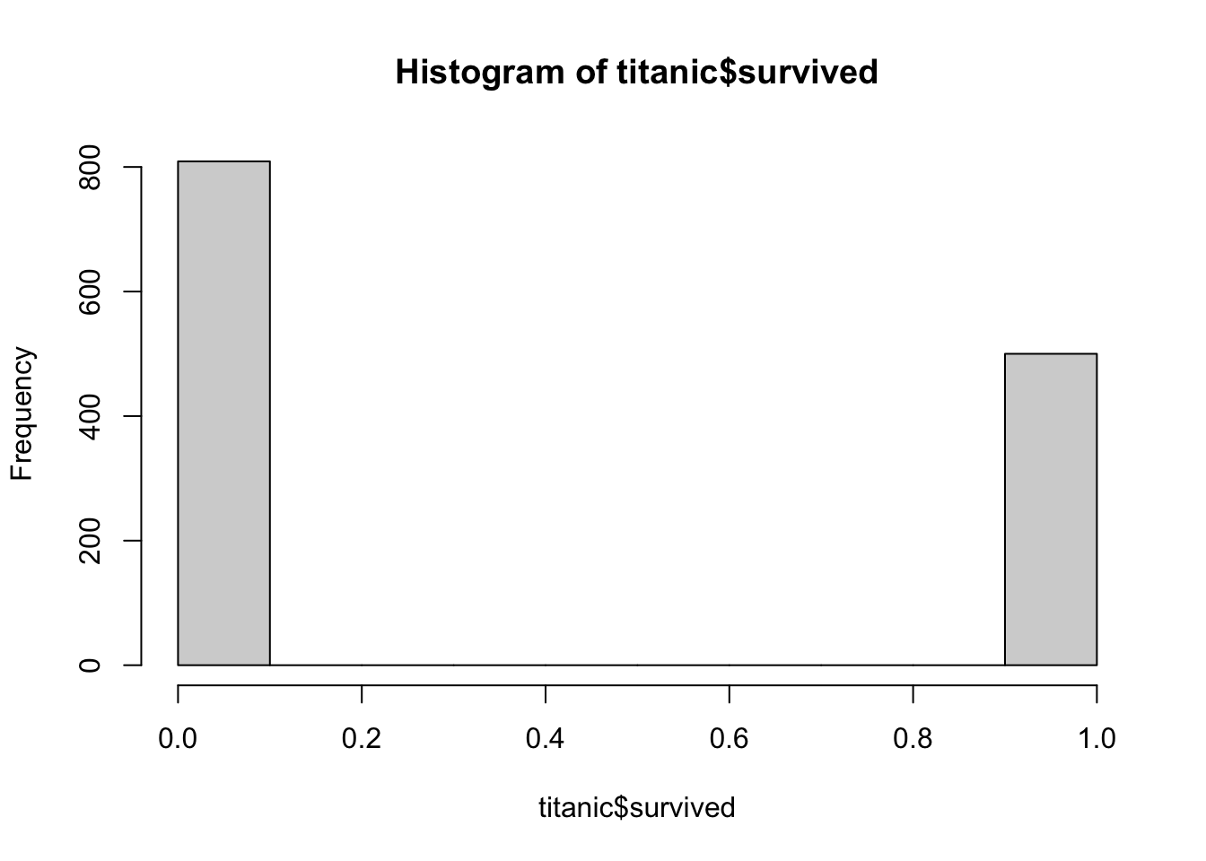

par(mfrow = c(1,1))

We can see that there is something seriously wrong with the residuals! One assumption for the lm is that the residuals and the response variable are normally distributed. Let’s inspect the distribution of the response variable

hist(titanic$survived)

table(titanic$survived)
## 
##   0   1 
## 809 500

Our response consists of 0s and 1s, so it is a binomial distribution. For binomial data we cannot use a lm because we need to restrict our values to be in the range of [0,1] (our model needs to predict probabilites).

The idea of generalized linear models is that we can use link (and inverse link functions) to transform the expected values into the range of our response.

All GLMs have:

a linear term to specify the desired dependency on explanatory variables (we already know this) \(y = a x + b x_2 + c\)
a link function to scale the linear term to the correct range of values for the distribution that was chosen. (this is new)
and a probability distribution that describes the model from which the dependent variable is generated. (this is also new – so far: normal = gaussian)

LM and GLMS – the three models you should know:

Type	R call	Properties
Linear regression (continuous data)	`lm(y ~ x)` or `glm(y~x, family = gaussian())`	Identity (no) link, normal distribution (family = gaussian) no inverse link
Logistic regression (1/0 or k out of n data)	`glm(y ~x, family = binomial)`	binomial distribution, logit link: \(log(p/(1-p))\)
		inverse link: \(exp(y)/(1 + exp(y))\)
Poisson regression (Count data)	`glm(y ~x, family = poisson)`	Poisson distribution, log link: \(log(lambda)\)
		inverse link: \(exp(y)\)

Model diagnostic (residual checks) cannot be done anymore by plotting the model. This can be only done for a lm! For glms we have to use the DHARMa package!

For more details on glms, see the chapter about glms in the advanced regression book.

10.1 Logistic Regression

For the binomial model we can use the logit link:

\[ logit(y) = a_0 +a_1*x \]

And the inverse link:

\[ y = \frac{1}{1+e^{-(a_0 + a_1) }} \]

You can interpret the glm outputs basically like lm outputs.

BUT: To get absolute response values, you have to transform the output with the inverse link function. For the logit, e.g. an intercept of 0 means a predicted value of 0.5.

Different overall statistics: no R², instead Pseudo R² = 1 - Residual deviance / Null deviance (deviance is based on the likelihood):

Let’s model the surivival data with sex as predictor.

# logistic regression with categorical predictor
m1 = glm(survived ~ sex, data = titanic, family = "binomial")
summary(m1)
## 
## Call:
## glm(formula = survived ~ sex, family = "binomial", data = titanic)
## 
## Coefficients:
##             Estimate Std. Error z value Pr(>|z|)    
## (Intercept)   0.9818     0.1040   9.437   <2e-16 ***
## sexmale      -2.4254     0.1360 -17.832   <2e-16 ***
## ---
## Signif. codes:  0 '***' 0.001 '**' 0.01 '*' 0.05 '.' 0.1 ' ' 1
## 
## (Dispersion parameter for binomial family taken to be 1)
## 
##     Null deviance: 1741.0  on 1308  degrees of freedom
## Residual deviance: 1368.1  on 1307  degrees of freedom
## AIC: 1372.1
## 
## Number of Fisher Scoring iterations: 4

Because we have 2 groups (female and male), the intercept will consist of one of the groups (female in this case because of alphabetical order - but you can change it as you wish). But this is not the surival probability of females! The coefficients are at the logit link function scale. So, we need to back transform it to the original scale:

# linear term for female
coef(m1)[1]
## (Intercept) 
##    0.981813
# survival probability for females
plogis(coef(m1)[1])
## (Intercept) 
##   0.7274678
# applies inverse logit function

To get the survival probabily for males, we have to sum the intercept to the coefficient of the difference (sexmale):

# linear term for male
coef(m1)[1] + coef(m1)[2]
## (Intercept) 
##   -1.443625
# survival probability
plogis(coef(m1)[1] + coef(m1)[2])
## (Intercept) 
##   0.1909846

You can get the same information with the predict function:

# predicted linear term
table(predict(m1))
## 
##  -1.4436252928589 0.981813020919314 
##               843               466
# predicted response
table(predict(m1, type = "response"))
## 
##  0.19098457888495 0.727467811158294 
##               843               466

Or nicer with the package effects

library(effects)
## Carregando pacotes exigidos: carData
## lattice theme set by effectsTheme()
## See ?effectsTheme for details.
plot(allEffects(m1))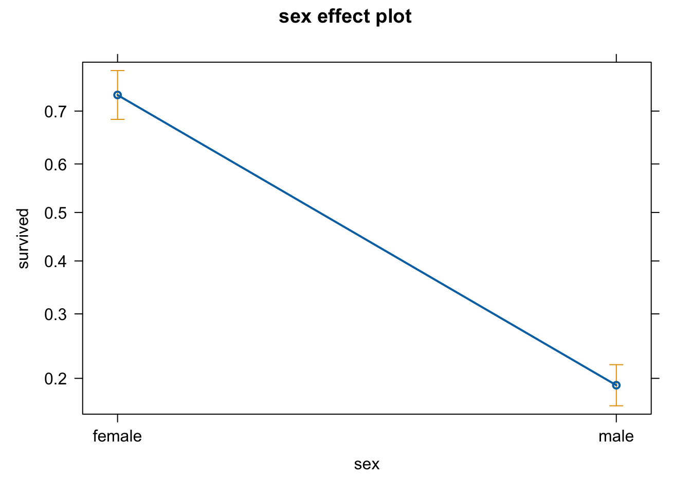

Adding age as a predictor

# more predictors
m2 = glm(survived ~ sex + age, titanic, family = binomial)
summary(m2)
## 
## Call:
## glm(formula = survived ~ sex + age, family = binomial, data = titanic)
## 
## Coefficients:
##              Estimate Std. Error z value Pr(>|z|)    
## (Intercept)  1.235414   0.192032   6.433 1.25e-10 ***
## sexmale     -2.460689   0.152315 -16.155  < 2e-16 ***
## age         -0.004254   0.005207  -0.817    0.414    
## ---
## Signif. codes:  0 '***' 0.001 '**' 0.01 '*' 0.05 '.' 0.1 ' ' 1
## 
## (Dispersion parameter for binomial family taken to be 1)
## 
##     Null deviance: 1414.6  on 1045  degrees of freedom
## Residual deviance: 1101.3  on 1043  degrees of freedom
##   (263 observations deleted due to missingness)
## AIC: 1107.3
## 
## Number of Fisher Scoring iterations: 4

plot(allEffects(m2))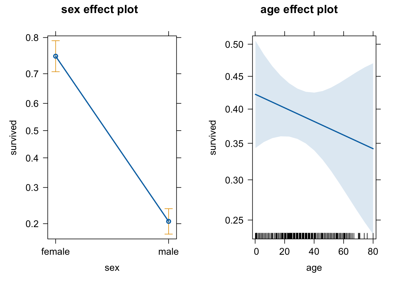

# Anova
anova(m2, test = "Chisq")
## Analysis of Deviance Table
## 
## Model: binomial, link: logit
## 
## Response: survived
## 
## Terms added sequentially (first to last)
## 
## 
##      Df Deviance Resid. Df Resid. Dev Pr(>Chi)    
## NULL                  1045     1414.6             
## sex   1  312.612      1044     1102.0   <2e-16 ***
## age   1    0.669      1043     1101.3   0.4133    
## ---
## Signif. codes:  0 '***' 0.001 '**' 0.01 '*' 0.05 '.' 0.1 ' ' 1

We can calculate the pseudo-R^2 by hand:

# Calculate Pseudo R2: 1 - Residual deviance / Null deviance
1 - 1101.3/1414.6 # Pseudo R2 of model
## [1] 0.221476

Or using the nice package called performance:

library(performance)
r2(m2)
## # R2 for Logistic Regression
##   Tjur's R2: 0.290

Let’s do a residual check:

# Model diagnostics
# do not use the plot(model) residual checks
# use DHARMa package
library(DHARMa)
## This is DHARMa 0.4.7. For overview type '?DHARMa'. For recent changes, type news(package = 'DHARMa')
res = simulateResiduals(m2)
plot(res)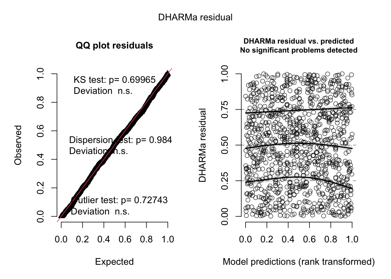

All good with our model now!

10.2 Poisson Regression

Poisson regression is used for count data. Properties of count data are:

no negative values,
only integers,
y ~ Poisson(lambda); where lambda = mean = variance,
log link function (lambda must be positive).

Example form the birdfeeding data from EcoData package

#head(birdfeeding)

plot(feeding ~ attractiveness, birdfeeding)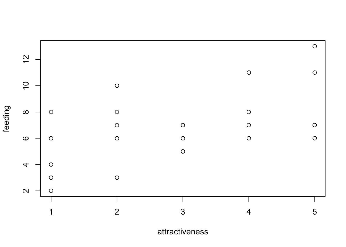


fit = glm(feeding ~ attractiveness, birdfeeding, family = "poisson")
summary(fit)
## 
## Call:
## glm(formula = feeding ~ attractiveness, family = "poisson", data = birdfeeding)
## 
## Coefficients:
##                Estimate Std. Error z value Pr(>|z|)    
## (Intercept)     1.47459    0.19443   7.584 3.34e-14 ***
## attractiveness  0.14794    0.05437   2.721  0.00651 ** 
## ---
## Signif. codes:  0 '***' 0.001 '**' 0.01 '*' 0.05 '.' 0.1 ' ' 1
## 
## (Dispersion parameter for poisson family taken to be 1)
## 
##     Null deviance: 25.829  on 24  degrees of freedom
## Residual deviance: 18.320  on 23  degrees of freedom
## AIC: 115.42
## 
## Number of Fisher Scoring iterations: 4

Plotting prediction:

plot(allEffects(fit))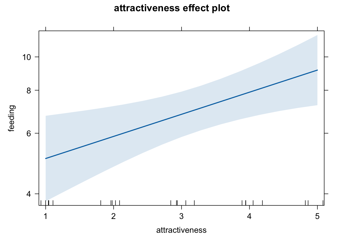

Checking residuals:

res = simulateResiduals(fit)
plot(res)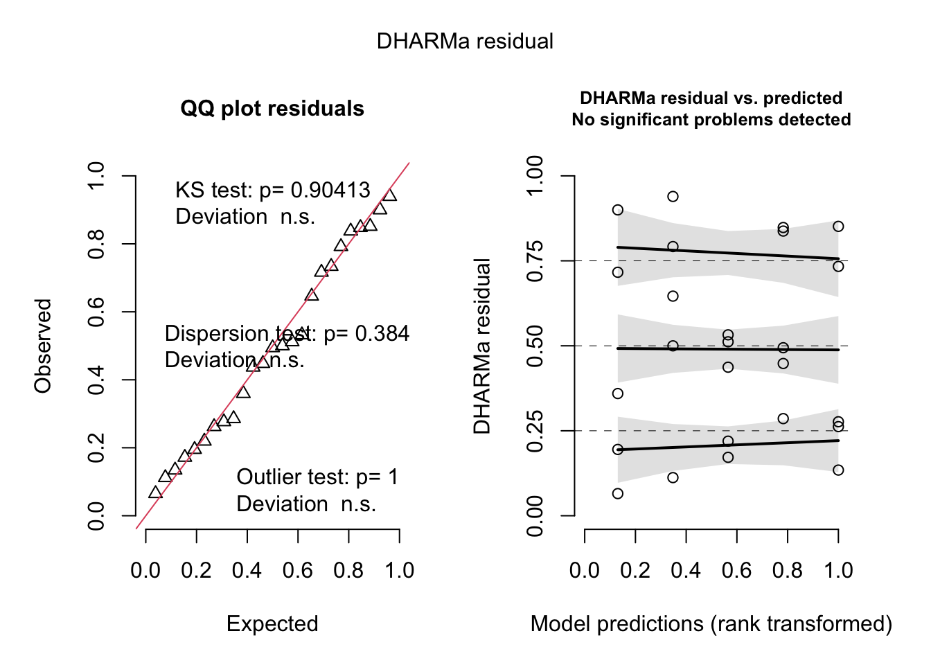

Normal versus Poisson distribution:

N(mean, sd). This means that fitting a normal distribution estimates a parameter for the variance (sd)
Poisson(lambda). lambda = mean = variance, This means that a Poisson regression does not fit a separate parameter for the variance!

So, the Poisson glm always assume that the variance is the mean, which is a strong assumption! In reality it can often occur that the variance is greater than expected (overdispersion) or smaller than expected (underdispersion). (this cannot happen for the lm because there we estimate a variance parameter (residual variance)). Overdispersion can have a HUGE influence on the MLEs and particularly on the p-values!

We can use the DHARMa package to check for Over or Underdispersion:

# test for overdispersion
testDispersion(fit, type = "PearsonChisq")
## Note that the chi2 test on Pearson residuals is biased for MIXED models towards underdispersion. Tests with alternative = two.sided or less are therefore not reliable. If you have random effects in your model, I recommend to test only with alternative = 'greater', i.e. test for overdispersion, or else use the DHARMa default tests which are unbiased. See help for details.
## 
##  Parametric dispersion test via mean Pearson-chisq statistic
## 
## data:  fit
## dispersion = 0.79322, df = 23, p-value = 0.5117
## alternative hypothesis: two.sided

Dispersion test is necessary for all poisson or proportion binomial models (k/n, number of success / number of trials). If you detect overdispersion in your model, you can use negative binomial distribution instead of poisson, and beta-binomial for the binomial. However, there are many nuances of data modeling that can lead to “overdispersion”, like misfit, zero-inflation or missing predictors. We suggest caution in dealing with that and you can read more about it at the book of the Advanced Regression Models course.