Multivariate statistics help us analyze datasets that have many variables at once. Instead of looking at each variable separately, we look at how they relate to each other and to the samples in our data. In ecology, for example, this helps us understand patterns in species composition or environmental variables. In this class, we’ll explore two common multivariate methods:
Ordination (to reduce complexity and visualize patterns) and
Clustering (to group similar observations).
11.1 Ordination:
11.1.1 PCA
We’ll start with Principal Component Analysis (PCA). This is a method to reduce the number of variables while keeping most of the variation in the data. It’s helpful for visualizing and summarizing complex datasets.The focus for the PCA is in the relationship among variables!
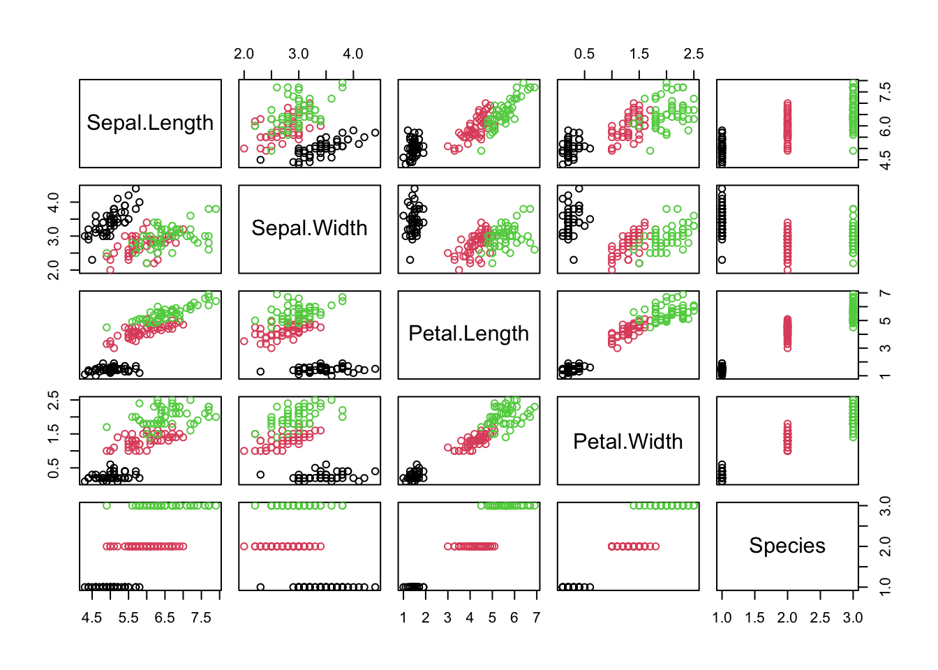
We’ll use the classic iris dataset, which has flower measurements for three iris species.
The pairs() plot shows the relationships between all pairs of variables, and how they differ among the species.
We run PCA using the four numeric columns and scale the variables to give them equal weight. The summary shows how much variance is explained by each principal component. The “cumulative proportion” shows how much of the total variation is captured as we include more components.
pca =prcomp(iris[, 1:4], scale = T) # always set scale = T# when data is very skewed --> better transform e.g. logsummary(pca)## Importance of components:## PC1 PC2 PC3 PC4## Standard deviation 1.7084 0.9560 0.38309 0.14393## Proportion of Variance 0.7296 0.2285 0.03669 0.00518## Cumulative Proportion 0.7296 0.9581 0.99482 1.00000# standard deviation^2 is variance!!!# cum prop of PC2 is the variance that is visualized in a biplot
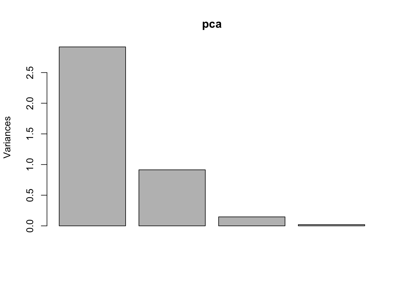
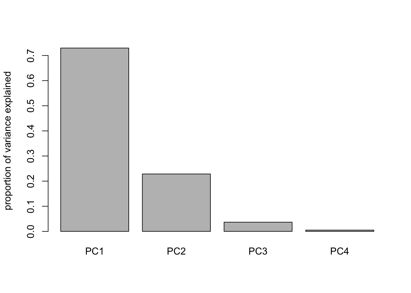
We can visualize the variance explained by each component. The scree plot shows the absolute variance, while the barplot shows the proportion explained by each component. These plots help us decide how many principal components to keep. Often, we look for a small number of components that explain most of the variation.
# absolute variance of each componentplot(pca) # see row1 of the summary(pca): (sd)^2 = variance
# rel variance of each componentbarplot(summary(pca)$importance[2, ], ylab="proportion of variance explained") # displays % of variance explained by PCs
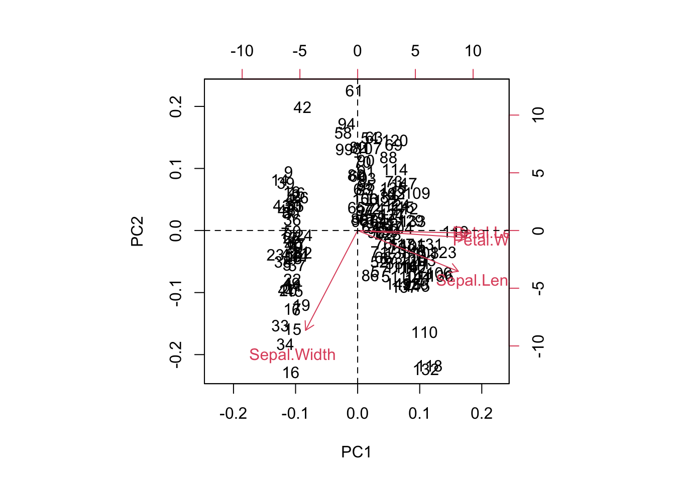
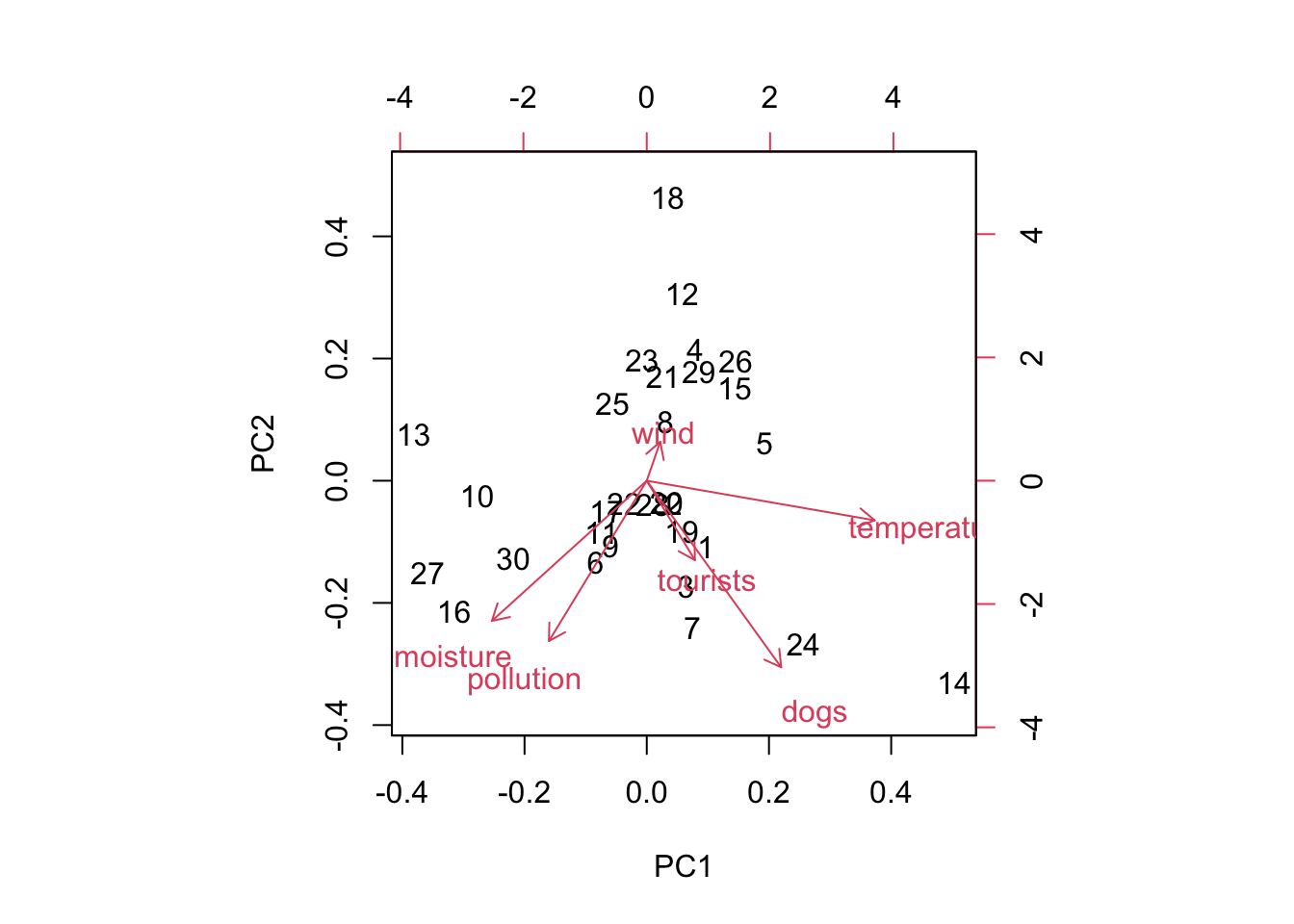
The biplot shows how the samples are positioned (numbers) in the reduced space (based on the first two components), and how the variables contribute to those components (red arrows).
biplot(pca) # displays PC1 and PC2 AND rotation (vectors) of the different variables AND observationsabline(v=0, lty="dashed") # adding lines in 0,0 to see betterabline(h=0, lty="dashed")
11.1.2 NMDS
Now let’s try Non-metric Multidimensional Scaling (NMDS). This is another type of ordination that works with distance (or dissimilarity) between samples (observations) instead of raw data. It’s often used in ecology to explore patterns in species composition across sites.
The focus on the NMDS is in the observations - the distance between observations given their properties (the variables).
We’ll use the dune dataset from the vegan package, which is a community dataset for plants in dunes. Each row is a site, and each column is a species. The values are species counts.
library(vegan)## Carregando pacotes exigidos: permute## Carregando pacotes exigidos: lattice#?vegandata("dune")str(dune) ## 'data.frame': 20 obs. of 30 variables:## $ Achimill: num 1 3 0 0 2 2 2 0 0 4 ...## $ Agrostol: num 0 0 4 8 0 0 0 4 3 0 ...## $ Airaprae: num 0 0 0 0 0 0 0 0 0 0 ...## $ Alopgeni: num 0 2 7 2 0 0 0 5 3 0 ...## $ Anthodor: num 0 0 0 0 4 3 2 0 0 4 ...## $ Bellpere: num 0 3 2 2 2 0 0 0 0 2 ...## $ Bromhord: num 0 4 0 3 2 0 2 0 0 4 ...## $ Chenalbu: num 0 0 0 0 0 0 0 0 0 0 ...## $ Cirsarve: num 0 0 0 2 0 0 0 0 0 0 ...## $ Comapalu: num 0 0 0 0 0 0 0 0 0 0 ...## $ Eleopalu: num 0 0 0 0 0 0 0 4 0 0 ...## $ Elymrepe: num 4 4 4 4 4 0 0 0 6 0 ...## $ Empenigr: num 0 0 0 0 0 0 0 0 0 0 ...## $ Hyporadi: num 0 0 0 0 0 0 0 0 0 0 ...## $ Juncarti: num 0 0 0 0 0 0 0 4 4 0 ...## $ Juncbufo: num 0 0 0 0 0 0 2 0 4 0 ...## $ Lolipere: num 7 5 6 5 2 6 6 4 2 6 ...## $ Planlanc: num 0 0 0 0 5 5 5 0 0 3 ...## $ Poaprat : num 4 4 5 4 2 3 4 4 4 4 ...## $ Poatriv : num 2 7 6 5 6 4 5 4 5 4 ...## $ Ranuflam: num 0 0 0 0 0 0 0 2 0 0 ...## $ Rumeacet: num 0 0 0 0 5 6 3 0 2 0 ...## $ Sagiproc: num 0 0 0 5 0 0 0 2 2 0 ...## $ Salirepe: num 0 0 0 0 0 0 0 0 0 0 ...## $ Scorautu: num 0 5 2 2 3 3 3 3 2 3 ...## $ Trifprat: num 0 0 0 0 2 5 2 0 0 0 ...## $ Trifrepe: num 0 5 2 1 2 5 2 2 3 6 ...## $ Vicilath: num 0 0 0 0 0 0 0 0 0 1 ...## $ Bracruta: num 0 0 2 2 2 6 2 2 2 2 ...## $ Callcusp: num 0 0 0 0 0 0 0 0 0 0 ...#?dunesummary(dune)## Achimill Agrostol Airaprae Alopgeni Anthodor ## Min. :0.0 Min. :0.0 Min. :0.00 Min. :0.00 Min. :0.00 ## 1st Qu.:0.0 1st Qu.:0.0 1st Qu.:0.00 1st Qu.:0.00 1st Qu.:0.00 ## Median :0.0 Median :1.5 Median :0.00 Median :0.00 Median :0.00 ## Mean :0.8 Mean :2.4 Mean :0.25 Mean :1.80 Mean :1.05 ## 3rd Qu.:2.0 3rd Qu.:4.0 3rd Qu.:0.00 3rd Qu.:3.25 3rd Qu.:2.25 ## Max. :4.0 Max. :8.0 Max. :3.00 Max. :8.00 Max. :4.00 ## Bellpere Bromhord Chenalbu Cirsarve Comapalu ## Min. :0.00 Min. :0.00 Min. :0.00 Min. :0.0 Min. :0.0 ## 1st Qu.:0.00 1st Qu.:0.00 1st Qu.:0.00 1st Qu.:0.0 1st Qu.:0.0 ## Median :0.00 Median :0.00 Median :0.00 Median :0.0 Median :0.0 ## Mean :0.65 Mean :0.75 Mean :0.05 Mean :0.1 Mean :0.2 ## 3rd Qu.:2.00 3rd Qu.:0.50 3rd Qu.:0.00 3rd Qu.:0.0 3rd Qu.:0.0 ## Max. :3.00 Max. :4.00 Max. :1.00 Max. :2.0 Max. :2.0 ## Eleopalu Elymrepe Empenigr Hyporadi Juncarti ## Min. :0.00 Min. :0.0 Min. :0.0 Min. :0.00 Min. :0.00 ## 1st Qu.:0.00 1st Qu.:0.0 1st Qu.:0.0 1st Qu.:0.00 1st Qu.:0.00 ## Median :0.00 Median :0.0 Median :0.0 Median :0.00 Median :0.00 ## Mean :1.25 Mean :1.3 Mean :0.1 Mean :0.45 Mean :0.90 ## 3rd Qu.:1.00 3rd Qu.:4.0 3rd Qu.:0.0 3rd Qu.:0.00 3rd Qu.:0.75 ## Max. :8.00 Max. :6.0 Max. :2.0 Max. :5.00 Max. :4.00 ## Juncbufo Lolipere Planlanc Poaprat Poatriv ## Min. :0.00 Min. :0.0 Min. :0.0 Min. :0.0 Min. :0.00 ## 1st Qu.:0.00 1st Qu.:0.0 1st Qu.:0.0 1st Qu.:0.0 1st Qu.:0.00 ## Median :0.00 Median :2.0 Median :0.0 Median :3.0 Median :4.00 ## Mean :0.65 Mean :2.9 Mean :1.3 Mean :2.4 Mean :3.15 ## 3rd Qu.:0.00 3rd Qu.:6.0 3rd Qu.:3.0 3rd Qu.:4.0 3rd Qu.:5.00 ## Max. :4.00 Max. :7.0 Max. :5.0 Max. :5.0 Max. :9.00 ## Ranuflam Rumeacet Sagiproc Salirepe Scorautu ## Min. :0.0 Min. :0.0 Min. :0 Min. :0.00 Min. :0.0 ## 1st Qu.:0.0 1st Qu.:0.0 1st Qu.:0 1st Qu.:0.00 1st Qu.:2.0 ## Median :0.0 Median :0.0 Median :0 Median :0.00 Median :2.0 ## Mean :0.7 Mean :0.9 Mean :1 Mean :0.55 Mean :2.7 ## 3rd Qu.:2.0 3rd Qu.:0.5 3rd Qu.:2 3rd Qu.:0.00 3rd Qu.:3.0 ## Max. :4.0 Max. :6.0 Max. :5 Max. :5.00 Max. :6.0 ## Trifprat Trifrepe Vicilath Bracruta Callcusp ## Min. :0.00 Min. :0.00 Min. :0.0 Min. :0.00 Min. :0.0 ## 1st Qu.:0.00 1st Qu.:1.00 1st Qu.:0.0 1st Qu.:1.50 1st Qu.:0.0 ## Median :0.00 Median :2.00 Median :0.0 Median :2.00 Median :0.0 ## Mean :0.45 Mean :2.35 Mean :0.2 Mean :2.45 Mean :0.5 ## 3rd Qu.:0.00 3rd Qu.:3.00 3rd Qu.:0.0 3rd Qu.:4.00 3rd Qu.:0.0 ## Max. :5.00 Max. :6.00 Max. :2.0 Max. :6.00 Max. :4.0
First, let’s chose the distance/dissimilarity metric. We use here a Bray-Curtis dissimilarity matrix (default in the metaMDSfunction), which is commonly used for community data. It measures how different the species compositions are between sites.
The metaMDS function runs NMDS and tries to represent the distances between sites in 2D space as accurately as possible.
NMDS =metaMDS(dune)## Run 0 stress 0.1192678 ## Run 1 stress 0.1886532 ## Run 2 stress 0.1192678 ## ... Procrustes: rmse 1.258026e-05 max resid 3.164268e-05 ## ... Similar to previous best## Run 3 stress 0.1183186 ## ... New best solution## ... Procrustes: rmse 0.02027014 max resid 0.06496123 ## Run 4 stress 0.1183186 ## ... Procrustes: rmse 4.230384e-06 max resid 1.475206e-05 ## ... Similar to previous best## Run 5 stress 0.1192678 ## Run 6 stress 0.1809578 ## Run 7 stress 0.1889638 ## Run 8 stress 0.1808911 ## Run 9 stress 0.3680059 ## Run 10 stress 0.1183186 ## ... Procrustes: rmse 1.159455e-05 max resid 3.442588e-05 ## ... Similar to previous best## Run 11 stress 0.1183186 ## ... Procrustes: rmse 4.643337e-06 max resid 1.388314e-05 ## ... Similar to previous best## Run 12 stress 0.2361935 ## Run 13 stress 0.1192678 ## Run 14 stress 0.1192679 ## Run 15 stress 0.1183186 ## ... Procrustes: rmse 1.447333e-05 max resid 4.510486e-05 ## ... Similar to previous best## Run 16 stress 0.1192678 ## Run 17 stress 0.1192678 ## Run 18 stress 0.1192679 ## Run 19 stress 0.1808911 ## Run 20 stress 0.1808911 ## *** Best solution repeated 4 timesNMDS # gives information on NMDS: distance measure, stress (should be low)## ## Call:## metaMDS(comm = dune) ## ## global Multidimensional Scaling using monoMDS## ## Data: dune ## Distance: bray ## ## Dimensions: 2 ## Stress: 0.1183186 ## Stress type 1, weak ties## Best solution was repeated 4 times in 20 tries## The best solution was from try 3 (random start)## Scaling: centring, PC rotation, halfchange scaling ## Species: expanded scores based on 'dune'
The STRESS (Standard Residuals Sum of Squares), is a measure of how the sites positions in the bidimensional configuration deviates from the original distances (from the distance matrix). I can be used as a measure of how adequate is the analysis for the dataset. As a rule of thumb, we have:
stress < 0.05 great representation;
stress < 0.01 good ordination
stress < 0.2 reazonable ordination
stress > 0.2 - be suspicious
stress >= 0.3 ordination is abitrary (do not interpret it)
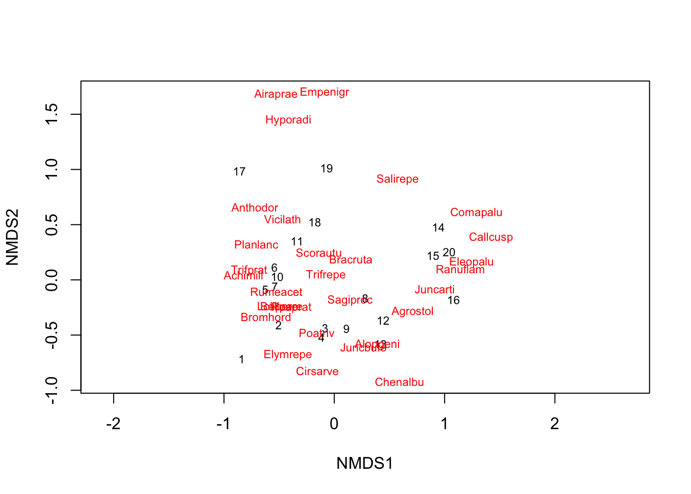
The NMDS plot shows how similar or different the sites are in terms of species composition. Sites that are close together have more similar species compositions.
ordiplot(NMDS, type ="t") #"t" = text for the species
Caution
Why we should be careful when interpreting patterns in ordination plots? Because it may find patterns even if the relationship between variables doesn’t exist:
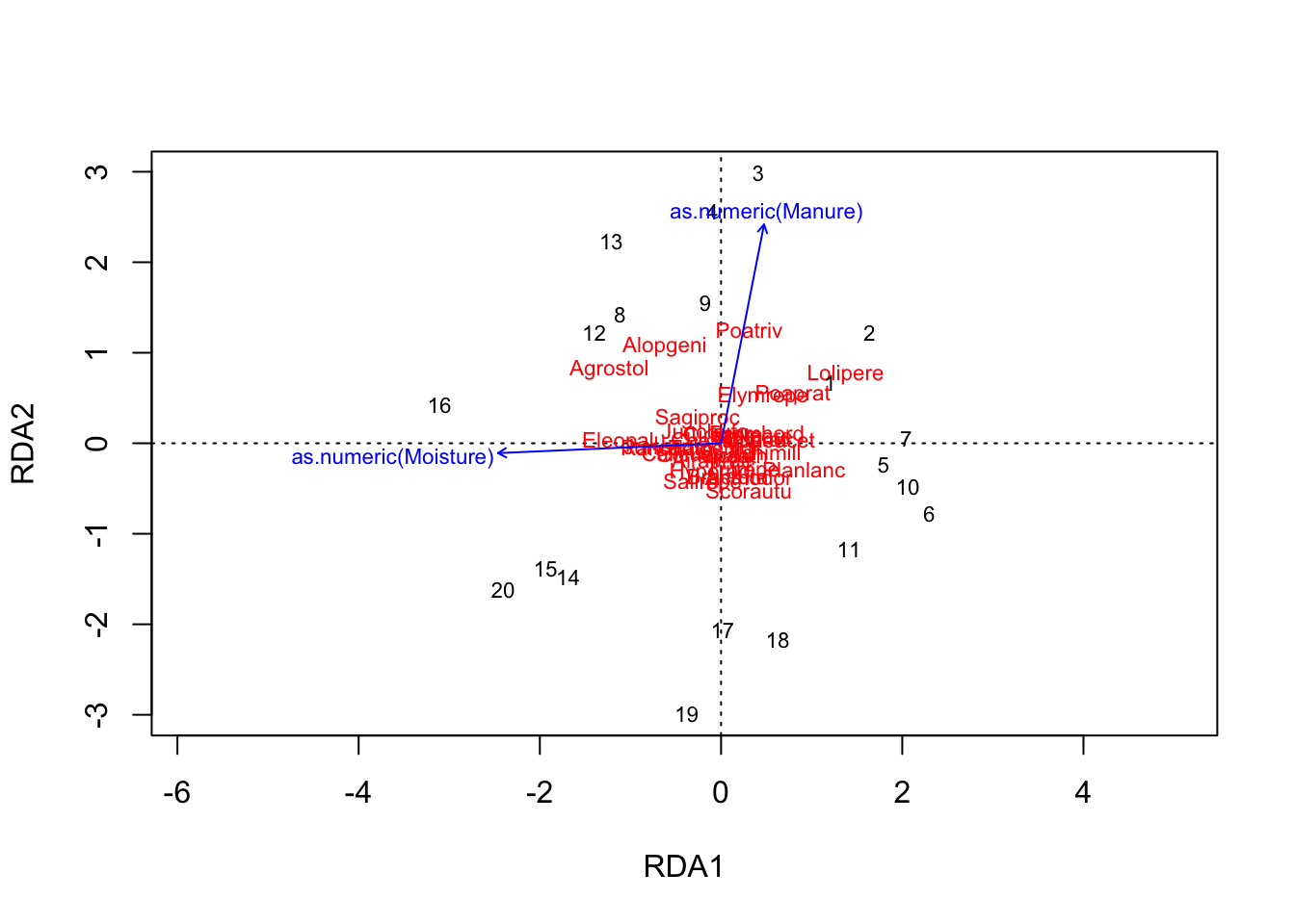
variance explained by the two variables = prop constrained = 37.09%
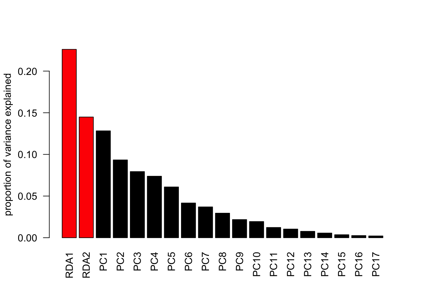
how much is explained by each RDA = see importance of components prop explained
PCs are the unconstrained axes
species scores = coordinates of species in the plot
site scores = coordinates of sites in the plot
biplot scores = coordinates of environmental variable vectors
barplot(summary(RDA)$cont$importance[2, ], las =2,col =c(rep ('red', 2), rep ('black', length(summary(RDA)$cont$importance[2, ])-2)),ylab="proportion of variance explained")
displays % of variance explained by PCs
11.3 Cluster analysis
Cluster analysis groups similar observations. It can be useful when we want to classify sites or samples based on their characteristics (variables).
There are two main types of clustering:
Hierarchical clustering: builds a tree (dendrogram) of nested clusters.
Non-hierarchical clustering (like K-means): partitions the data into a fixed number of clusters.
Comparing hiearchical and non-hiearchical clustering
Feature
Hierarchical
K-means (Non-hierarchical)
Number of groups
Decided after tree is built
Must be chosen before running
Input/ data type
Distance matrix
Raw (standardized) data
Result
Dendrogram (tree)
Cluster assignments
Flexibility
Can inspect different levels
Fixed number of groups
Sensitive to scaling?
Yes
Yes
Good for
Exploring nested group structure
Partitioning into defined clusters
Hierarchical clustering gives a full tree of nested groups, which is great for exploring data. K-means is simpler and faster, but you need to choose the number of groups first.
11.3.1 Hierarchical clustering
Let’s pretend we don’t know which species the iris individuals belong. We will use a hierarchical clustering technique to see how the individuals will be clustered by their morphological variables. We plot the results and then color individuals by their known species to see if the clustering could provide reliable classifications
For clustering you also need a dissimilarity matrix, here we are using the default from dist, the euclidian distance.
library(cluster) # clustering# example for distance matrixdist(iris[1:3, 1:4]) # creates a distance matrix (comparison of all possible sample pairs)## 1 2## 2 0.5385165 ## 3 0.5099020 0.3000000
Clustering and plotting.
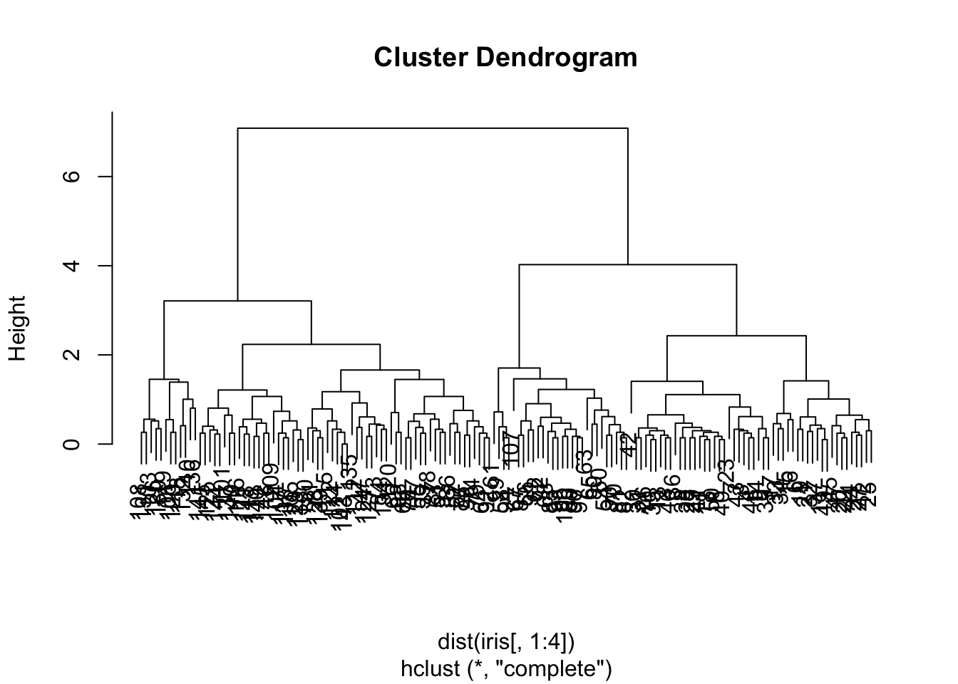
hc =hclust(dist(iris[, 1:4]))plot(hc)
THe default plot.hclust is ugly and don’t allow to color the tips (individuals). For that, we will use the package apefor phylogenetic analyses to get a pretty dendogram.
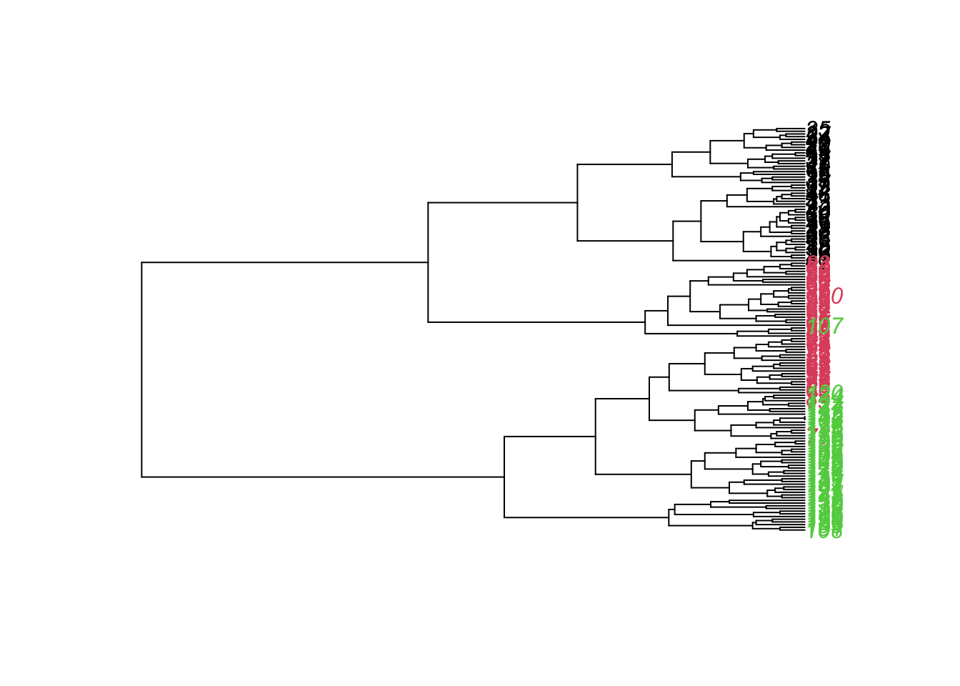
library(ape)new.hc <-as.phylo(hc, method ="ward.D2") # converts object type "hcclust" into type "phylo"plot(new.hc, tip.color =as.numeric(iris$Species))
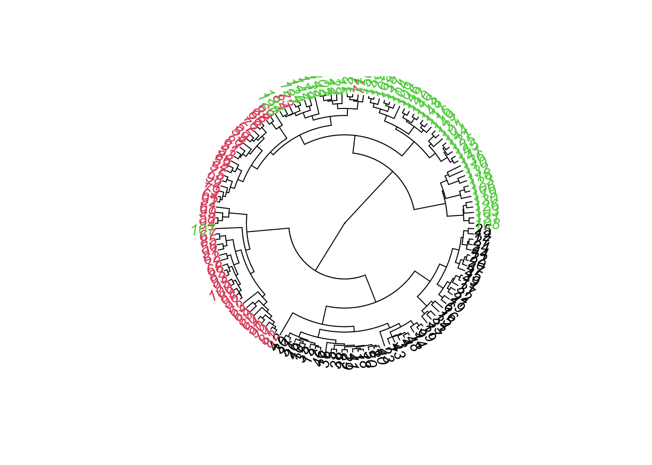
# change plotting type:plot(as.phylo(hc), tip.color =as.numeric(iris$Species), type ="fan")
The clustering algorithm did a good job in classifying the 3 species. Only 4 individuals (71,73,8,107) were wrongly attributed to a cluster formed mostly by another species. However, we see that the only species that had an isolated branch for itself was the setosa (black color), the other species had individuals spread in different braches.
11.3.2 Non-hiearchical clustering
The most common method for non-hierarchical clustering is K-means clustering, which partitions the data into a fixed number of groups. K-means clustering requires you to choose the number of clusters in advance. It works by assigning observations to the nearest cluster center, then updating the centers.
Note: K-means uses raw data (not a distance matrix), so we need to prepare the data differently.
We see again that the setosa species had all its individuals correctly clustered. The species versicolor and virginica presented some overlap.
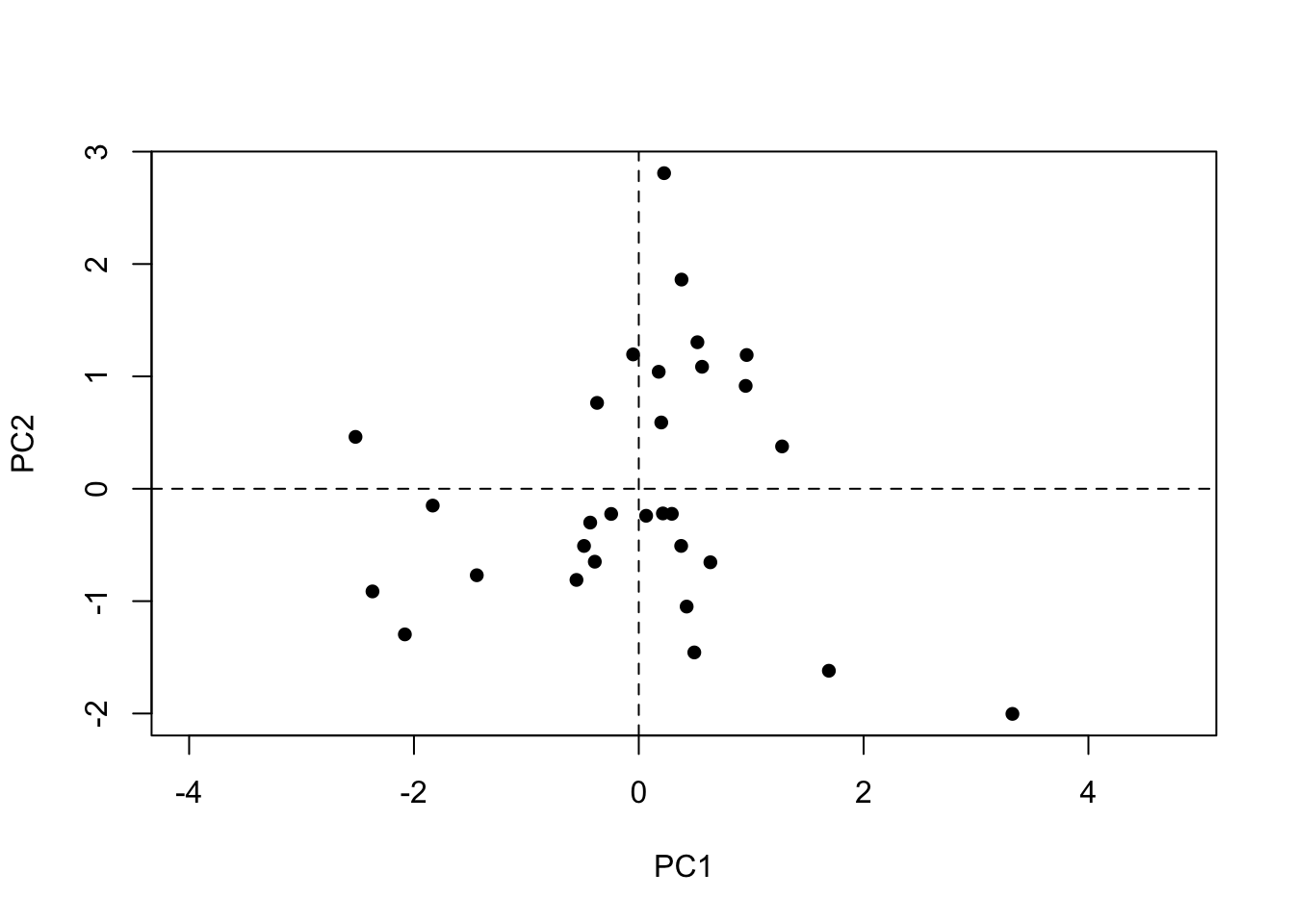
Let’s see the individuals that were wrongly attributed to another species in the pca plot (now using the function ordiplot from the vegan package):
wrong.class <-data.frame(cluster = cl$cluster, species = iris$Species)wrong.class$wrong <-"black"# creating column to color# color red for the wrong classificationwrong.class$wrong[wrong.class$species=="virginica"& wrong.class$cluster !=3| wrong.class$species=="versicolor"& wrong.class$cluster !=2] <-"red"ordiplot(pca, display="sites",) |>points("site", col=wrong.class$wrong, pch=16)abline(v=0, lty="dashed") # adding lines in 0,0 to see betterabline(h=0, lty="dashed")
This was just a brief overview of clustering methods. Here is a good online source for you to learn more.