2 Introduction to Machine Learning
Machine Learning (ML) is about training an algorithm that can perform certain tasks. The general steps to get the trained model are:
- Get some data (observations, the training data)
- Define what should be done with the data (the task)
- Find an (ML) algorithm that can perform the task
- Operationalize the goal through an error metric (the loss) that is to be minimized
- Train the algorithm to achieve a small loss on the data
- Evaluate the performance of the algorithm
Example
- data = airquality
- predict Ozone
- algorithm = lm
- loss = residual sum of squares
- m = lm(Ozone ~ ., data = airquality)
- could predict(m) to data or hold-out
The goal of this course is that you can answer the following questions:
- What tasks can we tackle?
- What algorithms exist, and how can they be set up, tuned, and modified?
- How do we define the loss, and how do we best train the algorithms?
- How do we evaluate model performance?
2.1 Machine Learning Tasks
Typically we can define roughly three types of ML tasks:
- Supervised learning
- Unsupervised learning
- Reinforcement learning
In supervised learning, you train an algorithm to predict something (categories = classification, or values = regression) from other data, and you provide it with correct examples of the task (the training data). The data you predict from are the features (the predictors, \(x\)), and the thing you predict is the response (\(y\)). Linear regression is an example of supervised learning. Given \(y = f(x)\) with \(x\) the input feature (e.g. precipitation), \(y\) the response (e.g. growth), and \(f\) an unknown function that maps \(x \rightarrow y\), the goal of supervised learning is to train an ML algorithm to approximate \(f\) from observed \((x_i, y_i)\) pairs.
In unsupervised learning, by contrast, you provide only the features and no examples of the correct output. Clustering techniques are a typical example (in the setting above, \(y\) would be unknown).
Reinforcement learning is a technique that mimics a game-like situation. The algorithm finds a solution through trial and error, receiving either rewards or penalties for each action. As in games, the goal is to maximize the rewards. We will talk more about this technique on the last day of the course.
For now, we will focus on the first two tasks, supervised and unsupervised learning (here a YouTube video explaining again the difference).
2.1.1 Test questions
In ML, predictors (the explanatory variables) are often called features:
In supervised learning the response (y) and the features (x) are known:
In unsupervised learning, only the features are known:
In reinforcement learning an agent (ML model) is trained by interacting with an environment:
Have a look at the two textbooks on ML (Elements of statistical learning and introduction to statistical learning) in our further readings at the end of the GRIPS course - which of the following statements is true?
2.2 Unsupervised Learning
In unsupervised learning, we want to identify patterns in the data without having any examples (supervision) of what the correct patterns or classes are. As an example, consider the iris dataset, which contains 150 observations of 4 floral traits:
iris = datasets::iris
colors = hcl.colors(3)
traits = as.matrix(iris[,1:4])
species = iris$Species
image(y = 1:4, x = 1:length(species), z = traits,
      ylab = "Floral trait", xlab = "Individual", yaxt = "n")
axis(2, at = 1:4, labels = colnames(traits), las = 1)
segments(50.5, 0, 50.5, 5, col = "black", lwd = 2)
segments(100.5, 0, 100.5, 5, col = "black", lwd = 2)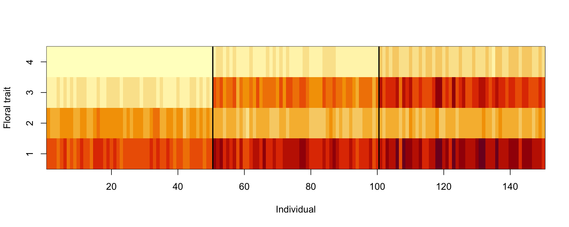
The observations come from 3 species, and because each species tends to have its own characteristic traits, the observations naturally form 3 clusters.
pairs(traits, pch = as.integer(species), col = colors[as.integer(species)])
However, imagine we don’t know what the species are — essentially the situation people faced in antiquity. They simply noticed that some plants had different flowers than others and decided to give them different names. This is the kind of process unsupervised learning carries out.
2.2.1 K-means Clustering
An example of an unsupervised learning algorithm is k-means clustering, one of the simplest and most popular unsupervised algorithms (we will return to it in the section on distance-based algorithms).
To start, you first specify the number of clusters (in our example, the number of species). Each cluster has a centroid, the location representing its center (here, what an average plant of a given species looks like). The algorithm begins by placing the centroids randomly. Each data point is then assigned to the cluster whose centroid is closest — more precisely, the assignment that increases the overall within-cluster sum of squares (the total squared distance of points to their centroid) the least. Once all points are assigned, the centroids are updated to the mean of their points. By repeating this procedure until the assignments no longer change, the algorithm finds (locally) optimal centroids and the points belonging to each cluster. Note that the result can depend on the initial centroid positions, so several different (locally) optimal solutions may exist.
The “k” in k-means refers to the number of clusters, and “means” refers to averaging the data points to find the centroids.
A typical pipeline for k-means clustering looks the same as for other algorithms: after visualizing the data, we fit a model, visualize the results, and assess the performance with a confusion matrix. Setting a fixed random seed (set.seed) ensures the results are reproducible.
set.seed(123)

#Reminder: traits = as.matrix(iris[,1:4]).

kc = kmeans(traits, 3)
print(kc)
K-means clustering with 3 clusters of sizes 50, 62, 38
Cluster means:
Sepal.Length Sepal.Width Petal.Length Petal.Width
1 5.006000 3.428000 1.462000 0.246000
2 5.901613 2.748387 4.393548 1.433871
3 6.850000 3.073684 5.742105 2.071053
Clustering vector:
[1] 1 1 1 1 1 1 1 1 1 1 1 1 1 1 1 1 1 1 1 1 1 1 1 1 1 1 1 1 1 1 1 1 1 1 1 1 1
[38] 1 1 1 1 1 1 1 1 1 1 1 1 1 2 2 3 2 2 2 2 2 2 2 2 2 2 2 2 2 2 2 2 2 2 2 2 2
[75] 2 2 2 3 2 2 2 2 2 2 2 2 2 2 2 2 2 2 2 2 2 2 2 2 2 2 3 2 3 3 3 3 2 3 3 3 3
[112] 3 3 2 2 3 3 3 3 2 3 2 3 2 3 3 2 2 3 3 3 3 3 2 3 3 3 3 2 3 3 3 2 3 3 3 2 3
[149] 3 2
Within cluster sum of squares by cluster:
[1] 15.15100 39.82097 23.87947
(between_SS / total_SS = 88.4 %)
Available components:
[1] "cluster" "centers" "totss" "withinss" "tot.withinss"
[6] "betweenss" "size" "iter" "ifault" Visualizing the results. Color codes true species identity, symbol shows cluster result.
plot(iris[c("Sepal.Length", "Sepal.Width")],
     col = colors[as.integer(species)], pch = kc$cluster,
     xlab = "Sepal length (cm)", ylab = "Sepal width (cm)")
points(kc$centers[, c("Sepal.Length", "Sepal.Width")],
       col = colors, pch = 1:3, cex = 3)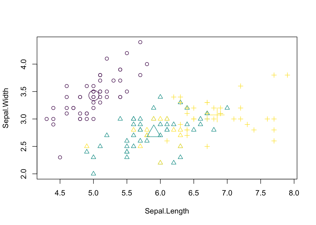
We see that there are some discrepancies. We can quantify them with a confusion matrix:
table(iris$Species, kc$cluster)
              1  2  3
  setosa     50  0  0
  versicolor  0 48  2
  virginica   0 14 36
A confusion matrix cross-tabulates the true groups (rows) against the predicted groups (columns). Counts on the diagonal are correct matches; off-diagonal counts are mistakes. A perfect result has all counts on the diagonal.
If you want to animate the clustering process, you could run
library(animation)

saveGIF(kmeans.ani(x = traits[,1:2], col = colors),
        interval = 1, ani.width = 800, ani.height = 800)
The elbow technique helps determine the best-suited number of clusters:
set.seed(123)

getSumSq = function(k){ kmeans(traits, k, nstart = 25)$tot.withinss }

# Perform the algorithm for different cluster sizes and retrieve the variance.
iris.kmeans1to10 = sapply(1:10, getSumSq)
plot(1:10, iris.kmeans1to10, type = "b", pch = 19, frame = FALSE,
     xlab = "Number of clusters K",
     ylab = "Total within-cluster sum of squares",
     col = c("black", "red", rep("black", 8)))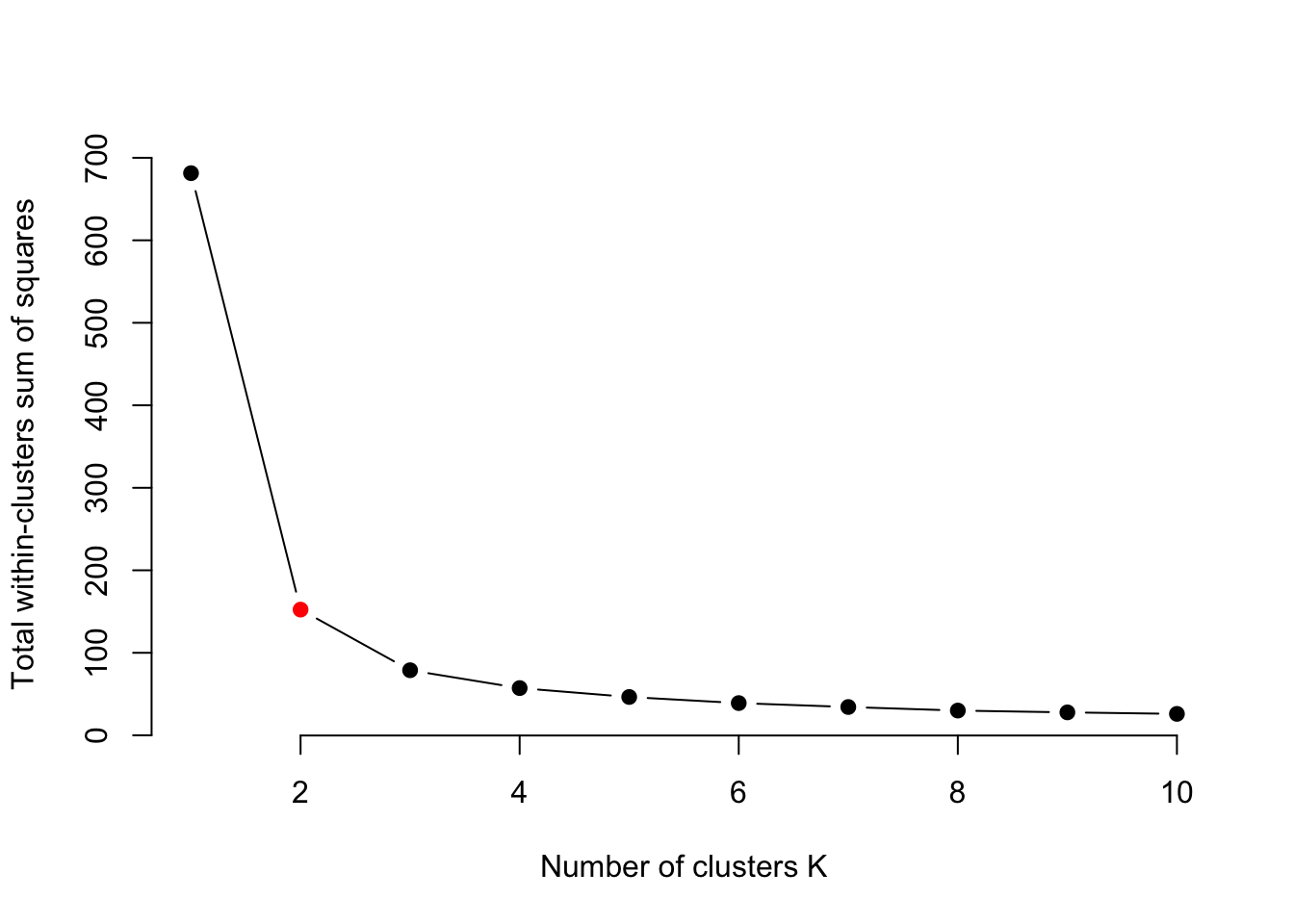
Often we prefer sparse models, and a higher k than necessary tends to overfit. We pick k at the “elbow” (kink) of the curve, where the sum of squares has dropped substantially but k is still low. Keep in mind that this is only a rule of thumb and can be misleading in some cases.
Information criteria such as AIC or BIC can be also used to select the number of clusters and control complexity.
2.3 Supervised Learning
The two most prominent branches of supervised learning are regression and classification. The distinction is simple: classification predicts a categorical variable (a class label), while regression predicts a continuous variable (a number).
2.3.1 Regression
The random forest (RF) algorithm is possibly the most widely used machine learning algorithm and works for both regression and classification. We will cover how it works in detail later; for now we just use it.
For now, we will go through a typical workflow for supervised regression: first we visualize the data, then we fit the model, and finally we visualize the results. We will again use the iris dataset. The goal is to predict Sepal.Length from the other variables (including species).
Fitting the model:
library(randomForest)
set.seed(123)
Sepal.Length is a numerical variable:
str(iris)'data.frame': 150 obs. of 5 variables:
$ Sepal.Length: num 5.1 4.9 4.7 4.6 5 5.4 4.6 5 4.4 4.9 ...
$ Sepal.Width : num 3.5 3 3.2 3.1 3.6 3.9 3.4 3.4 2.9 3.1 ...
$ Petal.Length: num 1.4 1.4 1.3 1.5 1.4 1.7 1.4 1.5 1.4 1.5 ...
$ Petal.Width : num 0.2 0.2 0.2 0.2 0.2 0.4 0.3 0.2 0.2 0.1 ...
$ Species : Factor w/ 3 levels "setosa","versicolor",..: 1 1 1 1 1 1 1 1 1 1 ...hist(iris$Sepal.Length, main = "", xlab = "Sepal length (cm)", col = "grey80")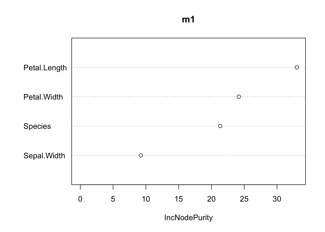
The random forest is used much like a linear regression model: we specify the features with the formula syntax (~ . means that all other variables are used as features):
m1 = randomForest(Sepal.Length ~ ., data = iris)   # ~.: Against all others.
print(m1)
Call:
 randomForest(formula = Sepal.Length ~ ., data = iris)
               Type of random forest: regression
                     Number of trees: 500
No. of variables tried at each split: 1

          Mean of squared residuals: 0.1389642
                    % Var explained: 79.6
The print-out reports the model’s out-of-bag (OOB) error. A random forest builds each tree on a random subsample of the data; the observations not used for a given tree are its “out-of-bag” data, and predicting them gives an honest performance estimate without a separate test set. For regression this is summarized as the mean of squared residuals and the % variance explained (similar to an \(R^2\)).
In statistics we would use a linear regression model:
mLM = lm(Sepal.Length~., data = iris)Like many other ML algorithms, the random forest is not directly interpretable: we don’t get coefficients that link the features to the response. We do, however, get the variable importance — similar in spirit to an ANOVA — which ranks how much each feature contributed to the predictions:
varImpPlot(m1, main = "")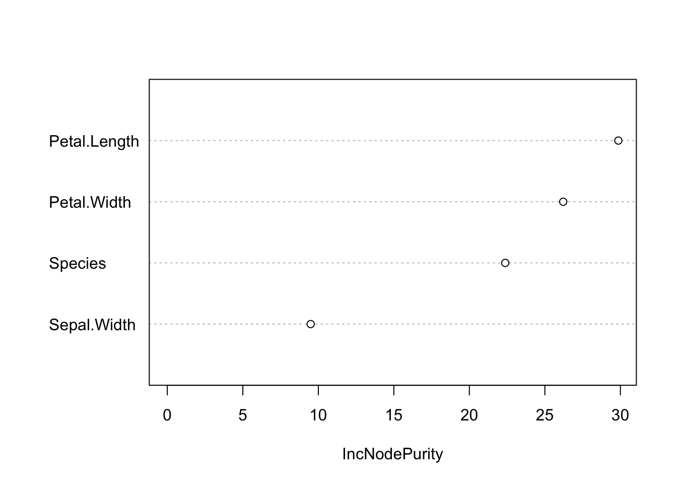
Variable importance (RF regression of sepal length): higher values indicate features that contribute more to reducing the prediction error.
Our linear model would report linear effects; however, the lm cannot match the flexibility of a random forest!
coef(mLM) (Intercept) Sepal.Width Petal.Length Petal.Width
2.1712663 0.4958889 0.8292439 -0.3151552
Speciesversicolor Speciesvirginica
-0.7235620 -1.0234978 Finally, we can use the model to make predictions with the predict method:
plot(predict(m1), iris$Sepal.Length,
     xlab = "Predicted sepal length (cm)", ylab = "Observed sepal length (cm)")
abline(0, 1)
A random forest is an ensemble of many decision trees. To inspect one of those individual trees, we can use a package from GitHub:
reprtree:::plot.getTree(m1, iris)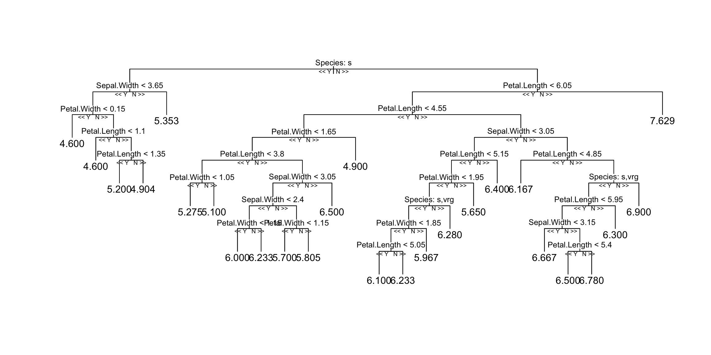
This is just one of the many trees; the random forest averages the predictions of all of them.
2.3.2 Classification
The random forest can also do classification. The workflow is the same as for regression, but now we can judge performance with the confusion matrix introduced earlier: it tabulates predicted classes against the true classes, so correct predictions land on the diagonal and mistakes off it.
Species is a factor with three levels (the three classes to predict):
str(iris)'data.frame': 150 obs. of 5 variables:
$ Sepal.Length: num 5.1 4.9 4.7 4.6 5 5.4 4.6 5 4.4 4.9 ...
$ Sepal.Width : num 3.5 3 3.2 3.1 3.6 3.9 3.4 3.4 2.9 3.1 ...
$ Petal.Length: num 1.4 1.4 1.3 1.5 1.4 1.7 1.4 1.5 1.4 1.5 ...
$ Petal.Width : num 0.2 0.2 0.2 0.2 0.2 0.4 0.3 0.2 0.2 0.1 ...
$ Species : Factor w/ 3 levels "setosa","versicolor",..: 1 1 1 1 1 1 1 1 1 1 ...Fitting the model (syntax is the same as for the regression task):
set.seed(123)
library(randomForest)
m1 = randomForest(Species ~ ., data = iris)
print(m1)
Call:
 randomForest(formula = Species ~ ., data = iris)
               Type of random forest: classification
                     Number of trees: 500
No. of variables tried at each split: 2

        OOB estimate of  error rate: 4.67%
Confusion matrix:
           setosa versicolor virginica class.error
setosa         50          0         0        0.00
versicolor      0         47         3        0.06
virginica 0 4 46 0.08varImpPlot(m1, main = "")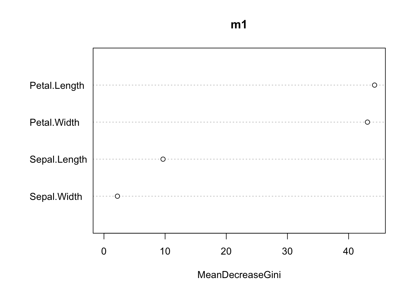
Predictions:
head(predict(m1)) 1 2 3 4 5 6
setosa setosa setosa setosa setosa setosa
Levels: setosa versicolor virginicaConfusion matrix:
table(predict(m1), as.integer(iris$Species))
              1  2  3
  setosa     50  0  0
  versicolor  0 47  4
  virginica   0  3 46
Our model made a few errors.
Visualizing the results:
plot(iris$Petal.Width, iris$Petal.Length, col = iris$Species,
     xlab = "Petal width (cm)", ylab = "Petal length (cm)")
mtext("A", side = 3, line = 0.5, adj = 0, font = 2, cex = 1.3)
plot(iris$Petal.Width, iris$Petal.Length, col = predict(m1),
     xlab = "Petal width (cm)", ylab = "Petal length (cm)")
mtext("B", side = 3, line = 0.5, adj = 0, font = 2, cex = 1.3)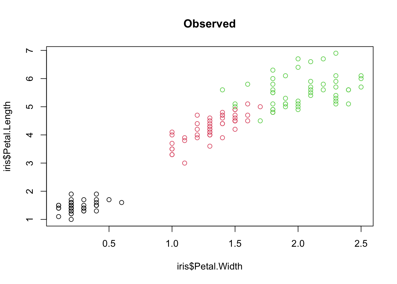
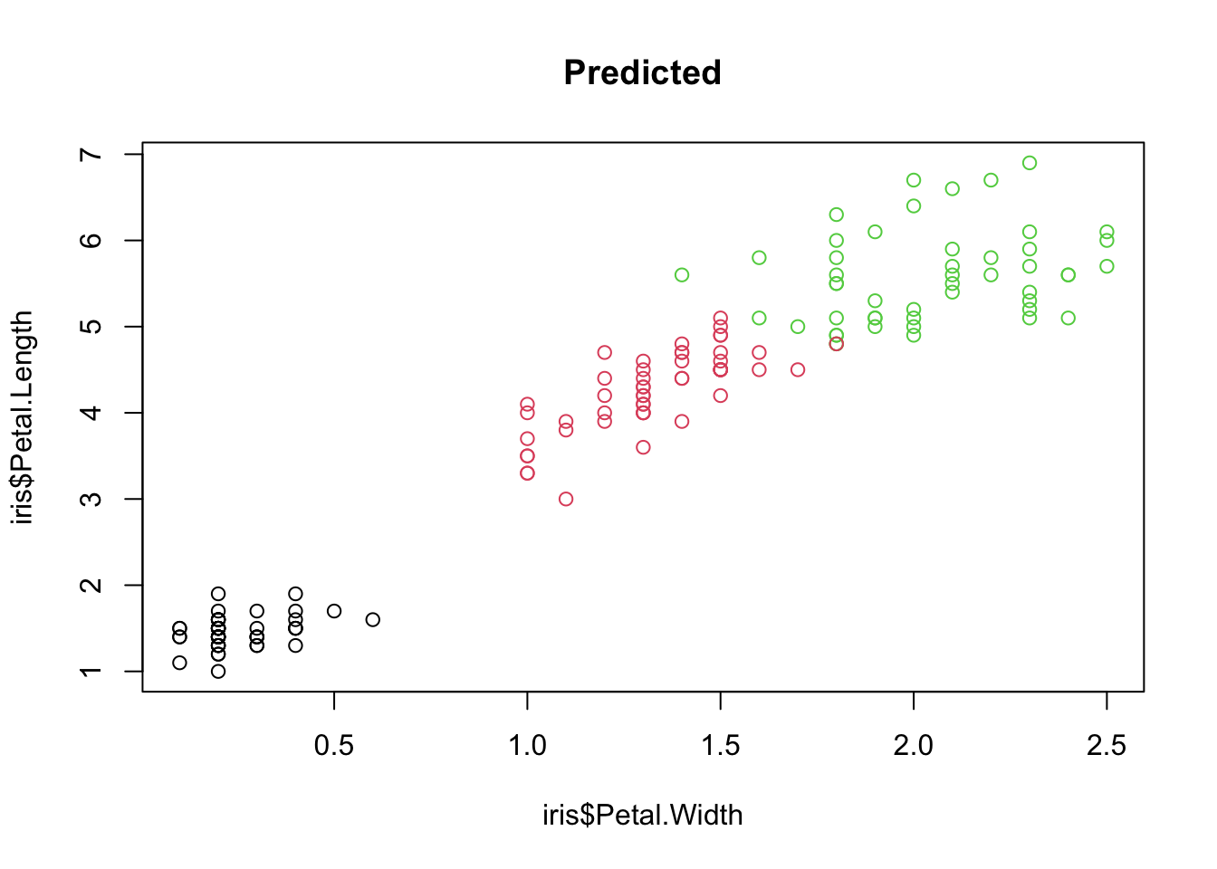
Species in petal trait space: (A) observed and (B) predicted by the random forest. Misclassifications appear where the colours differ between the two panels.
Visualizing one of the fitted models:
reprtree:::plot.getTree(m1, iris)
Confusion matrix:
| setosa | versicolor | virginica | |
|---|---|---|---|
| setosa | 50 | 0 | 0 |
| versicolor | 0 | 47 | 4 |
| virginica | 0 | 3 | 46 |
2.4 Exercise - Supervised Learning
Using a random forest on the iris dataset, which parameter would be more important (remember there is a function to check this) to predict Petal.Width?
2.4.0.1 Fit a random forest
Goal: fit a random forest, read its output, then switch the task from classification to regression by changing a single line.
A demonstration with the iris dataset:
library(randomForest)

# scale your features if possible (some ML algorithms converge faster with scaled features)
iris_scaled = iris
iris_scaled[,1:4] = scale(iris_scaled[,1:4])


model = randomForest(Species~., data = iris_scaled)
The random forest is not based on a specific data-generating model, so we do not get effect estimates that tell us how the input features affect the response:
# no summary method available
print(model)
Call:
 randomForest(formula = Species ~ ., data = iris_scaled)
               Type of random forest: classification
                     Number of trees: 500
No. of variables tried at each split: 2

        OOB estimate of  error rate: 4%
Confusion matrix:
           setosa versicolor virginica class.error
setosa         50          0         0        0.00
versicolor      0         47         3        0.06
virginica       0          3        47        0.06
The confusion matrix shows, for each species, where the model classifies correctly versus incorrectly on the out-of-bag (OOB) data. Recall that each tree is trained on a bootstrap sample of the data (sampling with replacement, so on average each bootstrap contains about 63% of the unique observations). The observations left out of a given bootstrap are used to validate that tree, and these errors are averaged over all trees in the forest.
While we don’t get effect estimates as in an lm, we do get the variable importance, which reports how important each predictor is:
varImpPlot(model, main = "")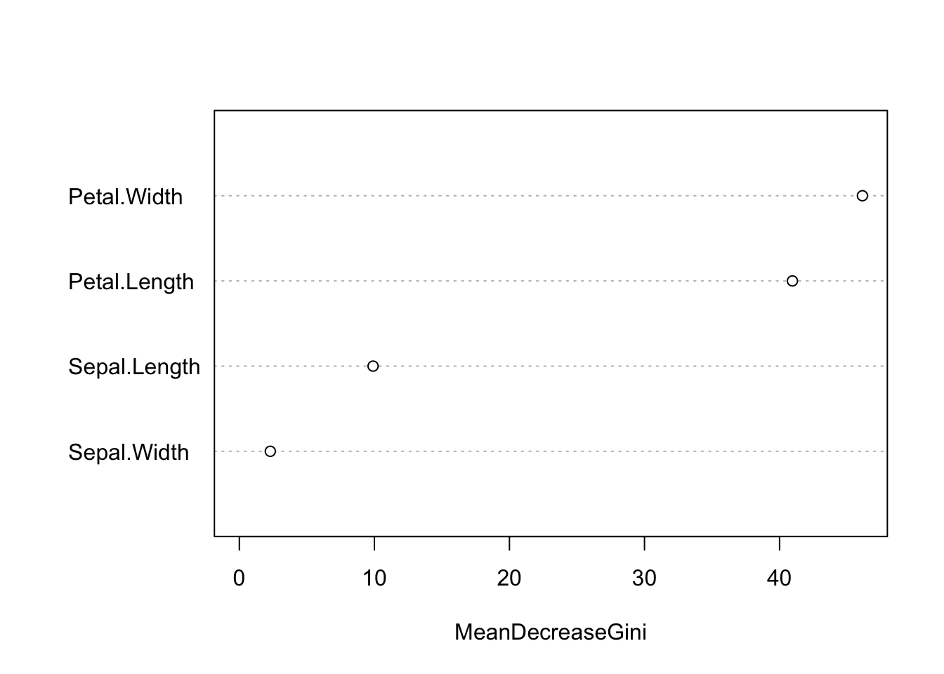
Variable importance for the random forest classifier trained on the scaled iris features.
Predictions
head(predict(model)) 1 2 3 4 5 6
setosa setosa setosa setosa setosa setosa
Levels: setosa versicolor virginicaThe model predicts the species class for each observation.
Performance:
table(predict(model), as.integer(iris$Species))
              1  2  3
  setosa     50  0  0
  versicolor  0 47  3
  virginica   0  3 47
Tasks
- Predict
Sepal.Lengthinstead ofSpecies, i.e. turn the classification problem into a regression. - Plot predicted vs. observed values. If the model is good, the points should fall close to the diagonal.
Quick check — once you predict Sepal.Length, which task is the random forest solving?
Random forest automatically infers the type of the task, so we don’t have to change much:
model = randomForest(Sepal.Length~., data = iris_scaled)The OOB error is now “% Var explained” which is very similar to an \(R^2\):
print(model)
Call:
 randomForest(formula = Sepal.Length ~ ., data = iris_scaled)
               Type of random forest: regression
                     Number of trees: 500
No. of variables tried at each split: 1

          Mean of squared residuals: 0.2039511
                    % Var explained: 79.47
Plot observed vs. predicted:
plot(iris_scaled$Sepal.Length, predict(model), xlim = c(-3, 3), ylim = c(-3, 3),
     xlab = "Observed sepal length (scaled)", ylab = "Predicted sepal length (scaled)")
abline(a = 0, b = 1)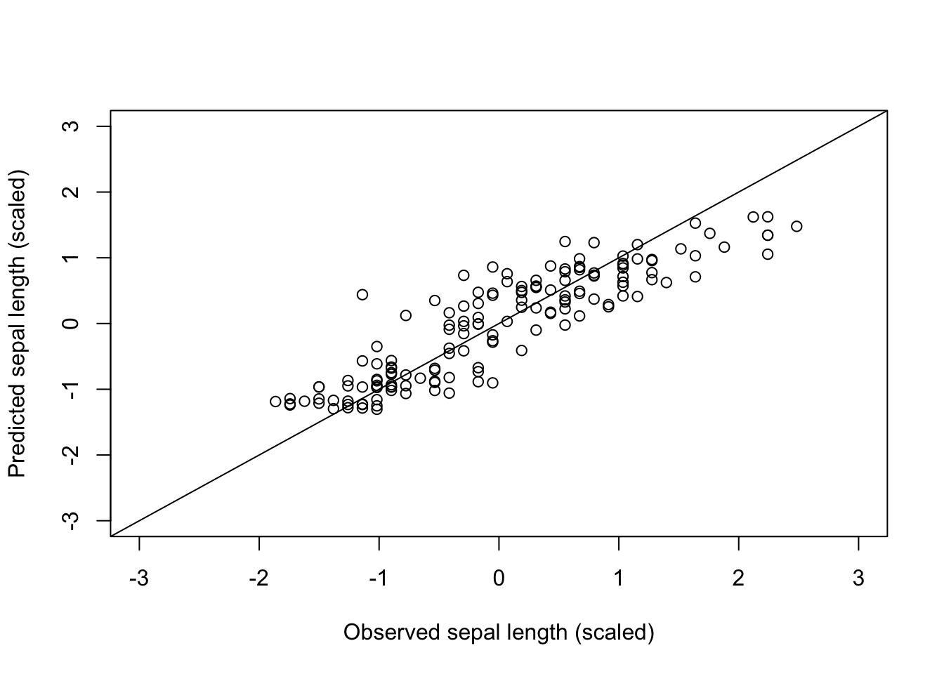
Predicted vs. observed (scaled) sepal length; points close to the 1:1 line indicate accurate predictions.
Calculate \(R^2\):
cor(iris_scaled$Sepal.Length, predict(model))^2[1] 0.79831962.5 Exercise - Train your first model and predict
The iris data above is small and clean, so almost any model works well. Let’s move to a larger, messier, ecological dataset — the plant–pollinator database — and walk through the core workflow: fit a model, then make predictions with it.
2.5.0.1 Train a random forest and make predictions
Goal: train your first random forest on a real dataset, read its performance, and make predictions — both as classes and as probabilities.
Working alone or in a group? This exercise works both ways, and either way you each write your own code:
- On your own: work through the tasks and note your answers to the discussion questions.
- In a group of 3–4: everyone fits and predicts independently, then you pool your answers and discuss together.
Prepare the data. We use only four trait predictors and a subsample of the observations — no feature engineering yet, that comes in later chapters:
library(EcoData)
library(randomForest)
library(missRanger)
library(dplyr)
set.seed(123)

data(plantPollinator_df)

# four trait predictors + the response; keep only the labelled observations
dat = plantPollinator_df |>
  select(diameter, corolla, tongue, body, interaction) |>
  filter(!is.na(interaction))

# impute the few missing trait values (only to remove NAs)
dat[, 1:4] = missRanger(dat[, 1:4], verbose = 0)
dat$interaction = as.factor(dat$interaction)

# the data set is large - subsample so a random forest fits in seconds
set.seed(123)
dat = dat[sample(nrow(dat), min(2000, nrow(dat))), ]
1. Fit the model. Train a random forest to predict whether a plant and a pollinator interact, and read its out-of-bag (OOB) error and confusion matrix:
set.seed(123)
rf = randomForest(interaction ~ ., data = dat)
print(rf)   # OOB error rate + confusion matrix
Call:
 randomForest(formula = interaction ~ ., data = dat)
               Type of random forest: classification
                     Number of trees: 500
No. of variables tried at each split: 2

        OOB estimate of  error rate: 4.05%
Confusion matrix:
     0  1 class.error
0 1912 14 0.007268951
1   67  7 0.905405405
2. Make predictions. A classifier can return two kinds of prediction — try both:
# (a) the predicted class: does this pair interact, yes or no?
pred_class = predict(rf)
head(pred_class)
2463 2511 10419 8718 12483 2986
0 0 0 0 0 0
Levels: 0 1# (b) the predicted probability of each class
pred_prob = predict(rf, type = "prob")
head(pred_prob) 0 1
2463 0.9195402 0.08045977
2511 1.0000000 0.00000000
10419 1.0000000 0.00000000
8718 1.0000000 0.00000000
12483 0.8709677 0.12903226
2986 0.9827586 0.01724138The class is simply the probability turned into a yes/no decision at a threshold (0.5 by default).
3. Hyperparameter teaser. Every algorithm has hyperparameters — settings you choose before training that change how it behaves (the random forest has ntree, mtry, nodesize, and more). Change one and refit, then see whether the OOB error moves:
set.seed(123)
rf2 = randomForest(interaction ~ ., data = dat, nodesize = 50)
print(rf2)
Call:
 randomForest(formula = interaction ~ ., data = dat, nodesize = 50)
               Type of random forest: classification
                     Number of trees: 500
No. of variables tried at each split: 2

        OOB estimate of  error rate: 3.7%
Confusion matrix:
     0 1 class.error
0 1926 0           0
1   74 0           1
Don’t worry yet about which values are good — that is exactly what the next chapter is about. For now it’s enough to see that these knobs exist and that they change the model.
Now discuss (or, if working alone, note down your answers):
- When would you rather have a probability than a hard class label? (Think about ranking the most likely interactions, or choosing your own threshold.)
- What does the confusion matrix tell you about which kinds of mistakes the model makes?
- Did changing the hyperparameter in step 3 move the OOB error — a little or a lot?
Quick check — what does predict(rf, type = "prob") return?
set.seed(123)
rf = randomForest(interaction ~ ., data = dat)

# classes and probabilities side by side for the first few observations
head(data.frame(class = predict(rf),
                predict(rf, type = "prob")))
class X0 X1
2463 0 0.9195402 0.08045977
2511 0 1.0000000 0.00000000
10419 0 1.0000000 0.00000000
8718 0 1.0000000 0.00000000
12483 0 0.8709677 0.12903226
2986 0 0.9827586 0.01724138# turning probabilities into classes with a 0.5 threshold reproduces the classes
prob_positive = predict(rf, type = "prob")[, 2]
manual_class = ifelse(prob_positive > 0.5, levels(dat$interaction)[2],
levels(dat$interaction)[1])
head(manual_class) 2463 2511 10419 8718 12483 2986
"0" "0" "0" "0" "0" "0" Probabilities are more informative than a bare class: they let you rank candidate interactions and choose a threshold that fits your goal (e.g. be more cautious before predicting an interaction). The confusion matrix shows whether the errors are mostly false positives or false negatives. Changing nodesize (or another hyperparameter) shifts the OOB error a little — why and how to choose these values is the subject of the next chapter.