Before we specialize on any tuning, it is important to understand that machine learning always consists of a pipeline of actions, illustrated here on the Titanic dataset.
The typical machine learning workflow consists of:
Data cleaning and exploration (EDA = explorative data analysis) for example with tidyverse.
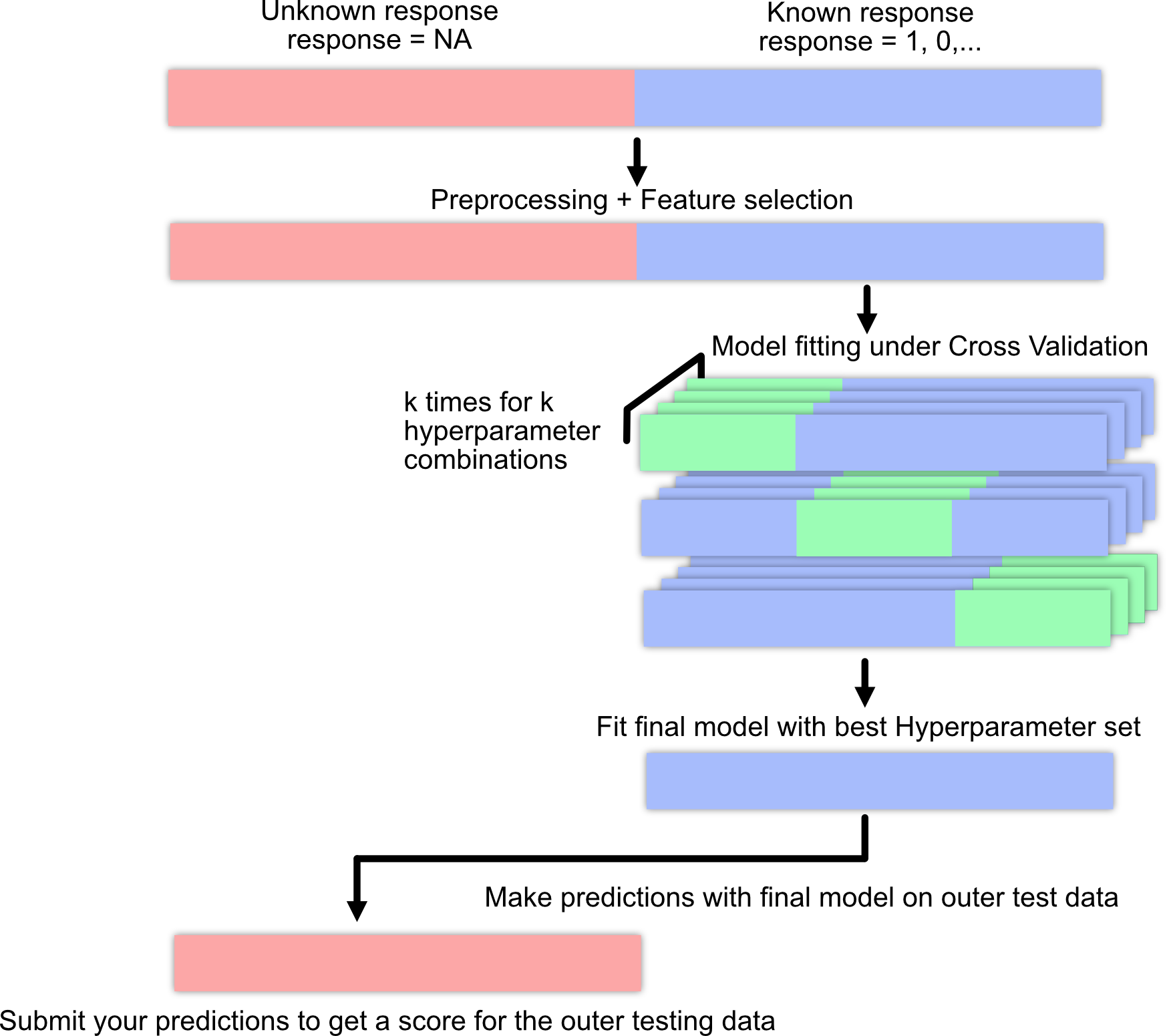
Preprocessing and feature selection.
Splitting data set into training and test set for evaluation.
Model fitting.
Model evaluation.
New predictions
Machine Learning pipeline
In the following example, we use tidyverse, a collection of R packages for data science / data manipulation mainly developed by Hadley Wickham.
dplyr and tidyverse
The dplyr package is part of a framework called tidyverse. Unique features of the tidyverse are the pipe |> operator and tibble objects.
The |> operator:
Applying several functions in sequence on an object often results in uncountable/confusing number of round brackets:
library(tidyverse)
── Attaching core tidyverse packages ──────────────────────── tidyverse 2.0.0 ──
✔ dplyr     1.2.1     ✔ readr     2.2.0
✔ forcats   1.0.1     ✔ stringr   1.6.0
✔ ggplot2   4.0.3     ✔ tibble    3.3.1
✔ lubridate 1.9.5     ✔ tidyr     1.3.2
✔ purrr     1.2.2
── Conflicts ────────────────────────────────────────── tidyverse_conflicts() ──
✖ dplyr::filter() masks stats::filter()
✖ dplyr::lag()    masks stats::lag()
ℹ Use the conflicted package (<http://conflicted.r-lib.org/>) to force all conflicts to become errors
max(mean(range(c(5, 3, 2, 1))))
[1] 3
The pipe operator simplifies that by saying “apply the next function on the result of the current function”:
c(5, 3, 2, 1) |>range() |>mean() |>max()
[1] 3
Which is easier to write, read, and to understand!
tibble objects are just an extension of data.frames. In the course we will use mostly data.frames, so it is better to transform the tibbles back to data.frames:
Another good reference is “R for data science” by Hadley Wickham: .
For this lecture you need the Titanic data set provided by us (via the EcoData package).
You can find it in GRIPS (datasets.RData in the data set and submission section) or at http://132.199.73.15:8500 (VPN for University of Regensburg is required!).
Motivation - We want a model to predict the survival probability of new passengers.
We have split the data set into training and an outer test/prediction data sets (the test/prediction split has one column less than the train split, as the response for the test/outer split is unknown).
The goal is to build a predictive model that can accurately predict the chances of survival for Titanic passengers!
NA = we don’t have information about the passenger, at the end, we will make predictions for these passengers!
Important: Preprocessing of the data must be done for the training and testing data together!!
4.1 Data preparation
Load necessary libraries:
library(tidyverse)
Load data set:
library(EcoData)data(titanic_ml)data = titanic_ml
Standard summaries:
str(data)
'data.frame':   1309 obs. of  13 variables:
 $ pclass   : int  2 1 3 3 3 3 3 1 3 1 ...
 $ survived : int  1 1 0 0 0 0 0 1 0 1 ...
 $ name     : chr  "Sinkkonen, Miss. Anna" "Woolner, Mr. Hugh" "Sage, Mr. Douglas Bullen" "Palsson, Master. Paul Folke" ...
 $ sex      : Factor w/ 2 levels "female","male": 1 2 2 2 2 2 2 1 1 1 ...
 $ age      : num  30 NA NA 6 30.5 38.5 20 53 NA 42 ...
 $ sibsp    : int  0 0 8 3 0 0 0 0 0 0 ...
 $ parch    : int  0 0 2 1 0 0 0 0 0 0 ...
 $ ticket   : Factor w/ 929 levels "110152","110413",..: 221 123 779 542 589 873 472 823 588 834 ...
 $ fare     : num  13 35.5 69.55 21.07 8.05 ...
 $ cabin    : Factor w/ 187 levels "","A10","A11",..: 1 94 1 1 1 1 1 1 1 1 ...
 $ embarked : Factor w/ 4 levels "","C","Q","S": 4 4 4 4 4 4 4 2 4 2 ...
 $ body     : int  NA NA NA NA 50 32 NA NA NA NA ...
 $ home.dest: Factor w/ 370 levels "","?Havana, Cuba",..: 121 213 1 1 1 1 322 350 1 1 ...
summary(data)
     pclass         survived             name          sex
 Min.   :1.000   Min.   :0.0000   Length   :1309   female:466
 1st Qu.:2.000   1st Qu.:0.0000   N.unique :1307   male  :843
 Median :3.000   Median :0.0000   N.blank  :   0
 Mean   :2.295   Mean   :0.3853   Min.nchar:  12
 3rd Qu.:3.000   3rd Qu.:1.0000   Max.nchar:  82
 Max.   :3.000   Max.   :1.0000
                 NAs    :655
      age              sibsp            parch            ticket
 Min.   : 0.1667   Min.   :0.0000   Min.   :0.000   CA. 2343:  11
 1st Qu.:21.0000   1st Qu.:0.0000   1st Qu.:0.000   1601    :   8
 Median :28.0000   Median :0.0000   Median :0.000   CA 2144 :   8
 Mean   :29.8811   Mean   :0.4989   Mean   :0.385   3101295 :   7
 3rd Qu.:39.0000   3rd Qu.:1.0000   3rd Qu.:0.000   347077  :   7
 Max.   :80.0000   Max.   :8.0000   Max.   :9.000   347082  :   7
 NAs    :263                                        (Other) :1261
      fare                     cabin      embarked      body
 Min.   :  0.000                  :1014    :  2    Min.   :  1.0
 1st Qu.:  7.896   C23 C25 C27    :   6   C:270    1st Qu.: 72.0
 Median : 14.454   B57 B59 B63 B66:   5   Q:123    Median :155.0
 Mean   : 33.295   G6             :   5   S:914    Mean   :160.8
 3rd Qu.: 31.275   B96 B98        :   4            3rd Qu.:256.0
 Max.   :512.329   C22 C26        :   4            Max.   :328.0
 NAs    :1         (Other)        : 271            NAs    :1188
                home.dest
                     :564
 New York, NY        : 64
 London              : 14
 Montreal, PQ        : 10
 Cornwall / Akron, OH:  9
 Paris, France       :  9
 (Other)             :639
The name variable consists of 1309 unique factors (there are 1309 observations…) and could be now transformed. If you are interested in how to do that, take a look at the following box.
Feature engineering of the name variable
length(unique(data$name))
[1] 1307
However, there is a title in each name. Let’s extract the titles:
We will extract all names and split each name after each comma “,”.
We will split the second split of the name after a point “.” and extract the titles.
# A tibble: 18 × 2
   f                n
   <fct>        <int>
 1 Capt             1
 2 Col              4
 3 Don              1
 4 Dona             1
 5 Dr               8
 6 Jonkheer         1
 7 Lady             1
 8 Major            2
 9 Master          61
10 Miss           260
11 Mlle             2
12 Mme              1
13 Mr             757
14 Mrs            197
15 Ms               2
16 Rev              8
17 Sir              1
18 the Countess     1
We will combine titles with low occurrences into one title, which we can easily do with the forcats package.
We can count titles again to see the new number of titles:
titles2 |>fct_count()
# A tibble: 6 × 2
  f           n
  <fct>   <int>
1 officer    23
2 royal       6
3 Master     61
4 miss      262
5 mrs       200
6 Mr        757
Add new title variable to data set:
data = data |>mutate(title = titles2)
4.1.1 Imputation
Missing values (NAs) are a common problem in ML, and most algorithms cannot handle them. We deal with this through imputation — filling in the missing values. For example, the age variable has 20% NAs:
summary(data$age)
   Min. 1st Qu.  Median    Mean 3rd Qu.    Max.     NAs
 0.1667 21.0000 28.0000 29.8811 39.0000 80.0000     263
sum(is.na(data$age)) /nrow(data)
[1] 0.2009167
There are few options how to handle NAs:
Drop observations with NAs, however, we may lose many observations (not what we want!)
Imputation, fill the missing values
We impute (fill) the missing values, for example with the median age. However, age itself might depend on other variables such as sex, class and title. Thus, instead of filling the NAs with the overall median of the passengers, we want to fill the NAs with the median age of these groups so that the associations with the other groups are preserved (or in other words, that the new values are hopefully closer to the unknown true values).
In tidyverse we can “group” the data, i.e. we will nest the observations within categorical variables for which we assume that there may be an association with age (here: group_by after sex, pclass and title). After grouping, all operations (such as our median(age....)) will be done within the specified groups (to get better estimates of these missing NAs).
Later (tomorrow), we want to use Keras in our example, but it cannot handle factors and requires the data to be scaled.
Normally, one would do this for all predictors, but as we only show the pipeline here, we have sub-selected a bunch of predictors and do this only for them. We first scale the numeric predictors and change the factors with only two groups/levels into integers (this can be handled by Keras).
Factors with more than two levels should be one hot encoded (Make columns for every different factor level and write 1 in the respective column for every taken feature value and 0 else. For example: \(\{red, green, green, blue, red\} \rightarrow \{(0,0,1), (0,1,0), (0,1,0), (1,0,0), (0,0,1)\}\)):
one_title =model.matrix(~0+as.factor(title), data = data)colnames(one_title) =levels(data$title)one_sex =model.matrix(~0+as.factor(sex), data = data)colnames(one_sex) =levels(data$sex)one_pclass =model.matrix(~0+as.factor(pclass), data = data)colnames(one_pclass) =paste0("pclass", 1:length(unique(data$pclass)))
And we have to add the dummy encoded variables to the data set:
data =cbind(data.frame(survived= data$survived), one_title, one_sex, age = data$age2,fare = data$fare2, one_pclass)head(data)
4.2 Modelling
4.2.1 Split data for final predictions
The concepts behind training/validation splits, cross-validation, and hyperparameter tuning were covered in Section 3.3; here we simply apply them inside the pipeline. To tune and evaluate our models, we split the data into training and testing data. The testing data are the observations where the response is NA:
summary(data_sub$survived)
   Min. 1st Qu.  Median    Mean 3rd Qu.    Max.     NAs
 0.0000  0.0000  0.0000  0.3853  1.0000  1.0000     655
655 observations have NAs in our response variable, these are the observations for which we want to make predictions at the end of our pipeline.
Minimal number of observations allowed in a node (before the branching is canceled)
Using the plant-pollinator dataset (see Section A.3), we want to optimize nodesize in our RF using a simple CV. The task is to predict whether a plant and a pollinator interact, based on their traits.
Prepare the data:
library(EcoData)library(dplyr)library(missRanger)data(plantPollinator_df)data = plantPollinator_dfdata = data |>select(interaction, diameter, corolla, tongue, body)# data imputation without the response variable!data[,-1] =missRanger(data[,-1], verbose =0)data$interaction =as.factor(data$interaction)data_sub = datadata_new = data_sub[is.na(data_sub$interaction),] # for which we want to make predictions at the enddata_obs = data_sub[!is.na(data_sub$interaction),] # data with known response
Hints:
adjust the ‘type’ argument in the predict(…) method (the default is to predict classes)
when predicting probabilities, the randomForest will return a matrix, a column for each class, we are interested in the probability of an interaction (so the second column)
The multi-species SDM dataset requires some data tinkering. For example:
Think about oversampling the rare species
Aggregate human footprint variables and land cover variables
Modelling strategies:
random forest implementations have weights arguments that can be used to put higher weights on specific levels (e.g. the rare species?)
tune nodesize
The dataset is available for download on the submission server or here (for external participants)
Here is a minimal example of how to prepare the dataset, fit a simple model, and prepare a submission:
Prepare the data:
load("sdm.RData")library(missRanger)library(tidyverse)sdm_long |>summary()sdm_long[,-3] = sdm_long[,-3] |>mutate(across(everything(), ~ifelse(is.na(.), mean(., na.rm =TRUE), .)))train = sdm_long[!is.na(sdm_long$present), ]test = sdm_long[is.na(sdm_long$present), ]# naive sub sampling of the training data due to computational constraints / we loose rare species?!!!indices =sample.int(nrow(train), 5000)train$present =as.factor(train$present) # crucial if you use the ranger package!
Fit the model
library(ranger)set.seed(123)rf =ranger(present ~ ., data = train[indices, -c(1, 4)], # without community and survey IDclassification =TRUE, probability =TRUE, num.trees =100L) # only 100 trees to speed up the predictions of the test dataset# presence probability per community x species row:preds =predict(rf, data = test)$predictions[, 2]
library(cito)m =dnn(X =as.data.frame(trainXs), Y = Y_train, loss ="bernoulli", ce =FALSE, lr =0.1, epochs =200L )probs =predict(m, newdata = testXs, type ="response")