library(keras3)
Attaching package: 'keras3'The following objects are masked from 'package:tensorflow':
set_random_seed, shape# or library(torch)We can use TensorFlow directly from R (see Appendix B for an introduction to TensorFlow), and we could use this knowledge to implement a neural network in TensorFlow directly in R. However, this can be quite cumbersome. For simple problems, it is usually faster to use a higher-level API that helps us implement the machine learning models in TensorFlow. The most common of these is Keras.
Keras is a powerful framework for building and training neural networks with just a few lines of code. As of the end of 2018, Keras and TensorFlow are fully interoperable, allowing us to take advantage of the best of both.
The goal of this lesson is to familiarize you with Keras. If you have TensorFlow installed, you can find Keras inside TensorFlow: tf.keras. However, the RStudio team has built an R package on top of tf.keras that is more convenient to use. To load the Keras package, type
library(keras3)
Attaching package: 'keras3'The following objects are masked from 'package:tensorflow':
set_random_seed, shape# or library(torch)We build a small classifier to predict the three species of the iris data set. Load the necessary packages and data sets:
library(keras3)
library(tensorflow)
library(torch)
Attaching package: 'torch'The following object is masked from 'package:keras3':
as_iteratordata(iris)
head(iris) Sepal.Length Sepal.Width Petal.Length Petal.Width Species
1 5.1 3.5 1.4 0.2 setosa
2 4.9 3.0 1.4 0.2 setosa
3 4.7 3.2 1.3 0.2 setosa
4 4.6 3.1 1.5 0.2 setosa
5 5.0 3.6 1.4 0.2 setosa
6 5.4 3.9 1.7 0.4 setosaFor neural networks, it is beneficial to scale the predictors (scaling = centering and standardization, see ?scale). We also split our data into predictors (X) and response (Y = the three species).
X = scale(iris[,1:4])
Y = iris[,5]
Additionally, Keras/TensorFlow cannot handle factors and we have to create contrasts (one-hot encoding). To do so, we have to specify the number of categories. This can be tricky for a beginner, because in other programming languages like Python and C++, arrays start at zero. Thus, when we would specify 3 as number of classes for our three species, we would have the classes 0,1,2,3. Keep this in mind.
Y = keras3::to_categorical(as.integer(Y) - 1L, 3)
head(Y) # 3 columns, one for each level of the response.
[,1] [,2] [,3]
[1,] 1 0 0
[2,] 1 0 0
[3,] 1 0 0
[4,] 1 0 0
[5,] 1 0 0
[6,] 1 0 0After having prepared the data, we start now with the typical workflow in keras.
1. Initialize a sequential model in Keras:
model = keras_model_sequential(shape(4L))Torch users can skip this step.
A sequential Keras model is a higher order type of model within Keras and consists of one input and one output model.
2. Add hidden layers to the model (we will learn more about hidden layers during the next days).
When specifying the hidden layers, we also have to specify the shape and a so called activation function. You can think of the activation function as decision for what is forwarded to the next neuron (but we will learn more about it later). If you want to know this topic in even more depth, consider watching the videos presented in section @ref(basicMath).
The shape of the input is the number of predictors (here 4) and the shape of the output is the number of classes (here 3).
model |>
  layer_dense(units = 20L, activation = "relu") |>
  layer_dense(units = 20L, activation = "relu") |>
  layer_dense(units = 20L, activation = "relu") |>
  layer_dense(units = 3L, activation = "softmax")
The Torch syntax is very similar, we will give a list of layers to the “nn_sequential” function. Here, we have to specify the softmax activation function as an extra layer:
model_torch =
  nn_sequential(
    nn_linear(4L, 20L),
    nn_relu(),
    nn_linear(20L, 20L),
    nn_relu(),
    nn_linear(20L, 20L),
    nn_relu(),
    nn_linear(20L, 3L),
    nn_softmax(2)
)3. Compile the model with a loss function (here: cross entropy) and an optimizer (here: Adamax).
We will learn about other options later, so for now, do not worry about the “learning_rate” (“lr” in Torch or earlier in TensorFlow) argument, cross entropy or the optimizer.
model |>
  compile(loss = keras3::loss_categorical_crossentropy,
          keras3::optimizer_adamax(learning_rate = 0.001))
summary(model)
Model: "sequential"
┏━━━━━━━━━━━━━━━━━━━━━━━━━━━━━━━━━━━┳━━━━━━━━━━━━━━━━━━━━━━━━━━┳━━━━━━━━━━━━━━━┓
┃ Layer (type) ┃ Output Shape ┃ Param # ┃
┡━━━━━━━━━━━━━━━━━━━━━━━━━━━━━━━━━━━╇━━━━━━━━━━━━━━━━━━━━━━━━━━╇━━━━━━━━━━━━━━━┩
│ dense (Dense) │ (None, 20) │ 100 │
├───────────────────────────────────┼──────────────────────────┼───────────────┤
│ dense_1 (Dense) │ (None, 20) │ 420 │
├───────────────────────────────────┼──────────────────────────┼───────────────┤
│ dense_2 (Dense) │ (None, 20) │ 420 │
├───────────────────────────────────┼──────────────────────────┼───────────────┤
│ dense_3 (Dense) │ (None, 3) │ 63 │
└───────────────────────────────────┴──────────────────────────┴───────────────┘
Total params: 1,003 (3.92 KB)
Trainable params: 1,003 (3.92 KB)
Non-trainable params: 0 (0.00 B)plot(model)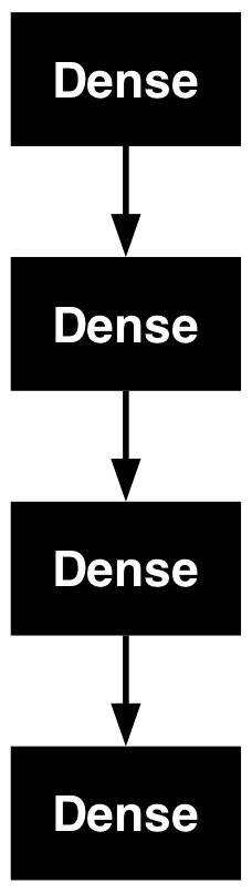
Specify optimizer and the parameters which will be trained (in our case the parameters of the network):
optimizer_torch = optim_adam(params = model_torch$parameters, lr = 0.001)4. Fit model in 30 iterations (epochs)
library(tensorflow)
library(keras3)


model_history =
  model |>
    fit(x = X, y = apply(Y, 2, as.integer), epochs = 30L,
        batch_size = 20L, shuffle = TRUE)
Epoch 1/30
8/8 - 0s - 30ms/step - loss: 1.0866
Epoch 2/30
8/8 - 0s - 1ms/step - loss: 1.0343
Epoch 3/30
8/8 - 0s - 1ms/step - loss: 0.9906
Epoch 4/30
8/8 - 0s - 1ms/step - loss: 0.9529
Epoch 5/30
8/8 - 0s - 1ms/step - loss: 0.9192
Epoch 6/30
8/8 - 0s - 1ms/step - loss: 0.8861
Epoch 7/30
8/8 - 0s - 1ms/step - loss: 0.8534
Epoch 8/30
8/8 - 0s - 1ms/step - loss: 0.8230
Epoch 9/30
8/8 - 0s - 1ms/step - loss: 0.7945
Epoch 10/30
8/8 - 0s - 1ms/step - loss: 0.7658
Epoch 11/30
8/8 - 0s - 1ms/step - loss: 0.7386
Epoch 12/30
8/8 - 0s - 1ms/step - loss: 0.7136
Epoch 13/30
8/8 - 0s - 1ms/step - loss: 0.6900
Epoch 14/30
8/8 - 0s - 1ms/step - loss: 0.6677
Epoch 15/30
8/8 - 0s - 1ms/step - loss: 0.6470
Epoch 16/30
8/8 - 0s - 1ms/step - loss: 0.6271
Epoch 17/30
8/8 - 0s - 1ms/step - loss: 0.6089
Epoch 18/30
8/8 - 0s - 1ms/step - loss: 0.5915
Epoch 19/30
8/8 - 0s - 1ms/step - loss: 0.5752
Epoch 20/30
8/8 - 0s - 1ms/step - loss: 0.5599
Epoch 21/30
8/8 - 0s - 1ms/step - loss: 0.5458
Epoch 22/30
8/8 - 0s - 1ms/step - loss: 0.5325
Epoch 23/30
8/8 - 0s - 1ms/step - loss: 0.5199
Epoch 24/30
8/8 - 0s - 1ms/step - loss: 0.5075
Epoch 25/30
8/8 - 0s - 1ms/step - loss: 0.4965
Epoch 26/30
8/8 - 0s - 1ms/step - loss: 0.4852
Epoch 27/30
8/8 - 0s - 1ms/step - loss: 0.4750
Epoch 28/30
8/8 - 0s - 1ms/step - loss: 0.4648
Epoch 29/30
8/8 - 0s - 1ms/step - loss: 0.4557
Epoch 30/30
8/8 - 0s - 1ms/step - loss: 0.4465In Torch, we jump directly to the training loop which we have to write on our own:
library(torch)
torch_manual_seed(321L)
set.seed(123)

# Calculate number of training steps.
epochs = 30
batch_size = 20
steps = round(nrow(X)/batch_size * epochs)

X_torch = torch_tensor(X)
Y_torch = torch_tensor(apply(Y, 1, which.max))

# Set model into training status.
model_torch$train()

log_losses = NULL

# Training loop.
for(i in 1:steps){
  # Get batch.
  indices = sample.int(nrow(X), batch_size)

  # Reset backpropagation.
  optimizer_torch$zero_grad()

  # Predict and calculate loss.
  pred = model_torch(X_torch[indices, ])
  loss = nnf_cross_entropy(pred, Y_torch[indices])

  # Backpropagation and weight update.
  loss$backward()
  optimizer_torch$step()

  log_losses[i] = as.numeric(loss)
}
5. Plot training history:
plot(model_history)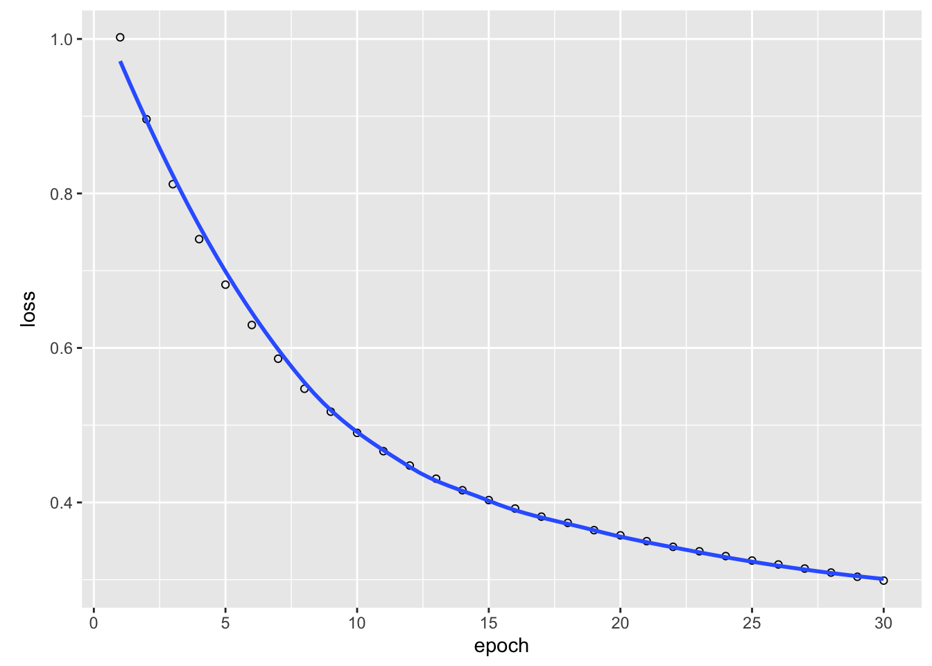
plot(log_losses, xlab = "steps", ylab = "loss", las = 1)
6. Create predictions:
predictions = predict(model, X) # Probabilities for each class.5/5 - 0s - 5ms/stepGet probabilities:
head(predictions) # Quasi-probabilities for each species. [,1] [,2] [,3]
[1,] 0.9702756 0.02589397 0.003830392
[2,] 0.9409620 0.05079169 0.008246413
[3,] 0.9674010 0.02887004 0.003729112
[4,] 0.9610399 0.03444652 0.004513510
[5,] 0.9769944 0.02032150 0.002684053
[6,] 0.9619896 0.03118199 0.006828349For each plant, we want to know for which species we got the highest probability:
preds = apply(predictions, 1, which.max)
print(preds)
[1] 1 1 1 1 1 1 1 1 1 1 1 1 1 1 1 1 1 1 1 1 1 1 1 1 1 1 1 1 1 1 1 1 1 1 1 1 1
[38] 1 1 1 1 1 1 1 1 1 1 1 1 1 3 3 3 2 3 2 3 2 3 2 2 3 2 3 2 3 2 2 3 2 3 3 3 3
[75] 3 3 3 3 3 2 2 2 2 3 2 3 3 3 2 2 2 3 2 2 2 2 2 3 2 2 3 3 3 3 3 3 2 3 3 3 3
[112] 3 3 3 3 3 3 3 3 3 3 3 3 3 3 3 3 3 3 3 3 3 3 3 3 3 3 3 3 3 3 3 3 3 3 3 3 3
[149] 3 3model_torch$eval()
preds_torch = model_torch(torch_tensor(X))
preds_torch = apply(preds_torch, 1, which.max)
print(preds_torch) [1] 1 1 1 1 1 1 1 1 1 1 1 1 1 1 1 1 1 1 1 1 1 1 1 1 1 1 1 1 1 1 1 1 1 1 1 1 1
[38] 1 1 1 1 1 1 1 1 1 1 1 1 1 2 2 3 2 2 2 2 2 2 2 2 2 2 2 2 2 2 2 2 2 2 2 2 2
[75] 2 2 2 3 2 2 2 2 2 2 2 2 2 2 2 2 2 2 2 2 2 2 2 2 2 2 3 3 3 3 3 3 2 3 3 3 3
[112] 3 3 3 3 3 3 3 3 2 3 3 3 3 3 3 3 3 3 3 3 3 3 2 2 3 3 3 2 3 3 3 3 3 3 3 3 3
[149] 3 27. Calculate Accuracy (how often we have been correct):
mean(preds == as.integer(iris$Species))[1] 0.8266667mean(preds_torch == as.integer(iris$Species))[1] 0.94666678. Plot predictions, to see if we have done a good job:
par(mfrow = c(1, 2))
plot(iris$Sepal.Length, iris$Petal.Length, col = iris$Species,
     main = "Observed")
plot(iris$Sepal.Length, iris$Petal.Length, col = preds,
     main = "Predicted")
Warning in par(oldpar): graphical parameter "cin" cannot be setWarning in par(oldpar): graphical parameter "cra" cannot be setWarning in par(oldpar): graphical parameter "csi" cannot be setWarning in par(oldpar): graphical parameter "cxy" cannot be setWarning in par(oldpar): graphical parameter "din" cannot be setWarning in par(oldpar): graphical parameter "page" cannot be setSo you see, building a neural network is very easy with Keras or Torch and you can already do it on your own.
We now build a regression for the airquality data set with Keras/Torch. We want to predict the variable “Ozone” (continuous).
Tasks:
Before we start, load and prepare the data set:
library(tensorflow)
library(keras3)


data = airquality

summary(data)
Ozone Solar.R Wind Temp
Min. : 1.00 Min. : 7.0 Min. : 1.700 Min. :56.00
1st Qu.: 18.00 1st Qu.:115.8 1st Qu.: 7.400 1st Qu.:72.00
Median : 31.50 Median :205.0 Median : 9.700 Median :79.00
Mean : 42.13 Mean :185.9 Mean : 9.958 Mean :77.88
3rd Qu.: 63.25 3rd Qu.:258.8 3rd Qu.:11.500 3rd Qu.:85.00
Max. :168.00 Max. :334.0 Max. :20.700 Max. :97.00
NAs :37 NAs :7
Month Day
Min. :5.000 Min. : 1.0
1st Qu.:6.000 1st Qu.: 8.0
Median :7.000 Median :16.0
Mean :6.993 Mean :15.8
3rd Qu.:8.000 3rd Qu.:23.0
Max. :9.000 Max. :31.0
data = data[complete.cases(data),]  # Remove NAs.
summary(data)
Ozone Solar.R Wind Temp
Min. : 1.0 Min. : 7.0 Min. : 2.30 Min. :57.00
1st Qu.: 18.0 1st Qu.:113.5 1st Qu.: 7.40 1st Qu.:71.00
Median : 31.0 Median :207.0 Median : 9.70 Median :79.00
Mean : 42.1 Mean :184.8 Mean : 9.94 Mean :77.79
3rd Qu.: 62.0 3rd Qu.:255.5 3rd Qu.:11.50 3rd Qu.:84.50
Max. :168.0 Max. :334.0 Max. :20.70 Max. :97.00
Month Day
Min. :5.000 Min. : 1.00
1st Qu.:6.000 1st Qu.: 9.00
Median :7.000 Median :16.00
Mean :7.216 Mean :15.95
3rd Qu.:9.000 3rd Qu.:22.50
Max. :9.000 Max. :31.00 x = scale(data[,2:6])
y = data[,1]library(tensorflow)
library(keras3)
model = keras_model_sequential(shape(5L))model |>
layer_dense(units = 20L, activation = "relu") |>
....
layer_dense(units = 1L, activation = "linear")model |>
layer_dense(units = 20L, activation = "relu") |>
layer_dense(units = 20L, activation = "relu") |>
layer_dense(units = 20L, activation = "relu") |>
layer_dense(units = 1L, activation = "linear")model |>
compile(loss = keras3::loss_mean_squared_error, optimizer_adamax(learning_rate = 0.05))What is the “mean_squared_error” loss?
model_history =
model |>
fit(x = x, y = as.numeric(y), epochs = 100L,
batch_size = 20L, shuffle = TRUE)Epoch 1/100
6/6 - 0s - 49ms/step - loss: 2345.1667
Epoch 2/100
6/6 - 0s - 2ms/step - loss: 810.1258
Epoch 3/100
6/6 - 0s - 1ms/step - loss: 452.4796
Epoch 4/100
6/6 - 0s - 1ms/step - loss: 417.2305
Epoch 5/100
6/6 - 0s - 1ms/step - loss: 358.7043
Epoch 6/100
6/6 - 0s - 1ms/step - loss: 332.7314
Epoch 7/100
6/6 - 0s - 1ms/step - loss: 322.0686
Epoch 8/100
6/6 - 0s - 1ms/step - loss: 303.3362
Epoch 9/100
6/6 - 0s - 1ms/step - loss: 310.0370
Epoch 10/100
6/6 - 0s - 1ms/step - loss: 308.5616
Epoch 11/100
6/6 - 0s - 1ms/step - loss: 292.0426
Epoch 12/100
6/6 - 0s - 1ms/step - loss: 302.5191
Epoch 13/100
6/6 - 0s - 1ms/step - loss: 280.6060
Epoch 14/100
6/6 - 0s - 1ms/step - loss: 288.2793
Epoch 15/100
6/6 - 0s - 1ms/step - loss: 274.7504
Epoch 16/100
6/6 - 0s - 1ms/step - loss: 273.7063
Epoch 17/100
6/6 - 0s - 1ms/step - loss: 270.2934
Epoch 18/100
6/6 - 0s - 1ms/step - loss: 262.2014
Epoch 19/100
6/6 - 0s - 1ms/step - loss: 260.7525
Epoch 20/100
6/6 - 0s - 1ms/step - loss: 267.9775
Epoch 21/100
6/6 - 0s - 1ms/step - loss: 249.7085
Epoch 22/100
6/6 - 0s - 1ms/step - loss: 249.0089
Epoch 23/100
6/6 - 0s - 2ms/step - loss: 248.1276
Epoch 24/100
6/6 - 0s - 1ms/step - loss: 239.8158
Epoch 25/100
6/6 - 0s - 1ms/step - loss: 236.2409
Epoch 26/100
6/6 - 0s - 1ms/step - loss: 240.3115
Epoch 27/100
6/6 - 0s - 1ms/step - loss: 228.4503
Epoch 28/100
6/6 - 0s - 1ms/step - loss: 227.5398
Epoch 29/100
6/6 - 0s - 1ms/step - loss: 222.5121
Epoch 30/100
6/6 - 0s - 1ms/step - loss: 220.8975
Epoch 31/100
6/6 - 0s - 1ms/step - loss: 230.1477
Epoch 32/100
6/6 - 0s - 2ms/step - loss: 211.8146
Epoch 33/100
6/6 - 0s - 1ms/step - loss: 221.8871
Epoch 34/100
6/6 - 0s - 1ms/step - loss: 211.1137
Epoch 35/100
6/6 - 0s - 1ms/step - loss: 209.1352
Epoch 36/100
6/6 - 0s - 1ms/step - loss: 205.8900
Epoch 37/100
6/6 - 0s - 2ms/step - loss: 200.1062
Epoch 38/100
6/6 - 0s - 1ms/step - loss: 198.2542
Epoch 39/100
6/6 - 0s - 1ms/step - loss: 194.9113
Epoch 40/100
6/6 - 0s - 1ms/step - loss: 196.8164
Epoch 41/100
6/6 - 0s - 1ms/step - loss: 187.6510
Epoch 42/100
6/6 - 0s - 1ms/step - loss: 188.5173
Epoch 43/100
6/6 - 0s - 1ms/step - loss: 183.9022
Epoch 44/100
6/6 - 0s - 1ms/step - loss: 188.9968
Epoch 45/100
6/6 - 0s - 1ms/step - loss: 180.1079
Epoch 46/100
6/6 - 0s - 1ms/step - loss: 178.0110
Epoch 47/100
6/6 - 0s - 1ms/step - loss: 181.3298
Epoch 48/100
6/6 - 0s - 1ms/step - loss: 176.2079
Epoch 49/100
6/6 - 0s - 1ms/step - loss: 171.3904
Epoch 50/100
6/6 - 0s - 1ms/step - loss: 172.9064
Epoch 51/100
6/6 - 0s - 1ms/step - loss: 166.1030
Epoch 52/100
6/6 - 0s - 1ms/step - loss: 165.2963
Epoch 53/100
6/6 - 0s - 1ms/step - loss: 166.2546
Epoch 54/100
6/6 - 0s - 1ms/step - loss: 158.7571
Epoch 55/100
6/6 - 0s - 1ms/step - loss: 163.7636
Epoch 56/100
6/6 - 0s - 1ms/step - loss: 163.0292
Epoch 57/100
6/6 - 0s - 1ms/step - loss: 149.0646
Epoch 58/100
6/6 - 0s - 1ms/step - loss: 156.5972
Epoch 59/100
6/6 - 0s - 1ms/step - loss: 150.8126
Epoch 60/100
6/6 - 0s - 1ms/step - loss: 152.5229
Epoch 61/100
6/6 - 0s - 1ms/step - loss: 144.8703
Epoch 62/100
6/6 - 0s - 1ms/step - loss: 145.6728
Epoch 63/100
6/6 - 0s - 1ms/step - loss: 140.4203
Epoch 64/100
6/6 - 0s - 1ms/step - loss: 144.5466
Epoch 65/100
6/6 - 0s - 1ms/step - loss: 135.1095
Epoch 66/100
6/6 - 0s - 1ms/step - loss: 137.0558
Epoch 67/100
6/6 - 0s - 1ms/step - loss: 160.8908
Epoch 68/100
6/6 - 0s - 1ms/step - loss: 141.7926
Epoch 69/100
6/6 - 0s - 1ms/step - loss: 126.3349
Epoch 70/100
6/6 - 0s - 1ms/step - loss: 141.3799
Epoch 71/100
6/6 - 0s - 1ms/step - loss: 123.8469
Epoch 72/100
6/6 - 0s - 1ms/step - loss: 136.1674
Epoch 73/100
6/6 - 0s - 2ms/step - loss: 119.1179
Epoch 74/100
6/6 - 0s - 1ms/step - loss: 122.0272
Epoch 75/100
6/6 - 0s - 1ms/step - loss: 112.6811
Epoch 76/100
6/6 - 0s - 1ms/step - loss: 120.1747
Epoch 77/100
6/6 - 0s - 1ms/step - loss: 121.7875
Epoch 78/100
6/6 - 0s - 1ms/step - loss: 118.6600
Epoch 79/100
6/6 - 0s - 1ms/step - loss: 108.1999
Epoch 80/100
6/6 - 0s - 1ms/step - loss: 111.9637
Epoch 81/100
6/6 - 0s - 1ms/step - loss: 106.5627
Epoch 82/100
6/6 - 0s - 1ms/step - loss: 113.0440
Epoch 83/100
6/6 - 0s - 1ms/step - loss: 129.7262
Epoch 84/100
6/6 - 0s - 1ms/step - loss: 121.7256
Epoch 85/100
6/6 - 0s - 1ms/step - loss: 94.6789
Epoch 86/100
6/6 - 0s - 1ms/step - loss: 106.9673
Epoch 87/100
6/6 - 0s - 1ms/step - loss: 104.2800
Epoch 88/100
6/6 - 0s - 2ms/step - loss: 93.4813
Epoch 89/100
6/6 - 0s - 1ms/step - loss: 95.9903
Epoch 90/100
6/6 - 0s - 1ms/step - loss: 96.4986
Epoch 91/100
6/6 - 0s - 1ms/step - loss: 92.8176
Epoch 92/100
6/6 - 0s - 1ms/step - loss: 91.7897
Epoch 93/100
6/6 - 0s - 1ms/step - loss: 88.2499
Epoch 94/100
6/6 - 0s - 1ms/step - loss: 89.5192
Epoch 95/100
6/6 - 0s - 2ms/step - loss: 83.3226
Epoch 96/100
6/6 - 0s - 1ms/step - loss: 85.7297
Epoch 97/100
6/6 - 0s - 1ms/step - loss: 85.2994
Epoch 98/100
6/6 - 0s - 1ms/step - loss: 85.8290
Epoch 99/100
6/6 - 0s - 1ms/step - loss: 99.0410
Epoch 100/100
6/6 - 0s - 1ms/step - loss: 90.8229plot(model_history)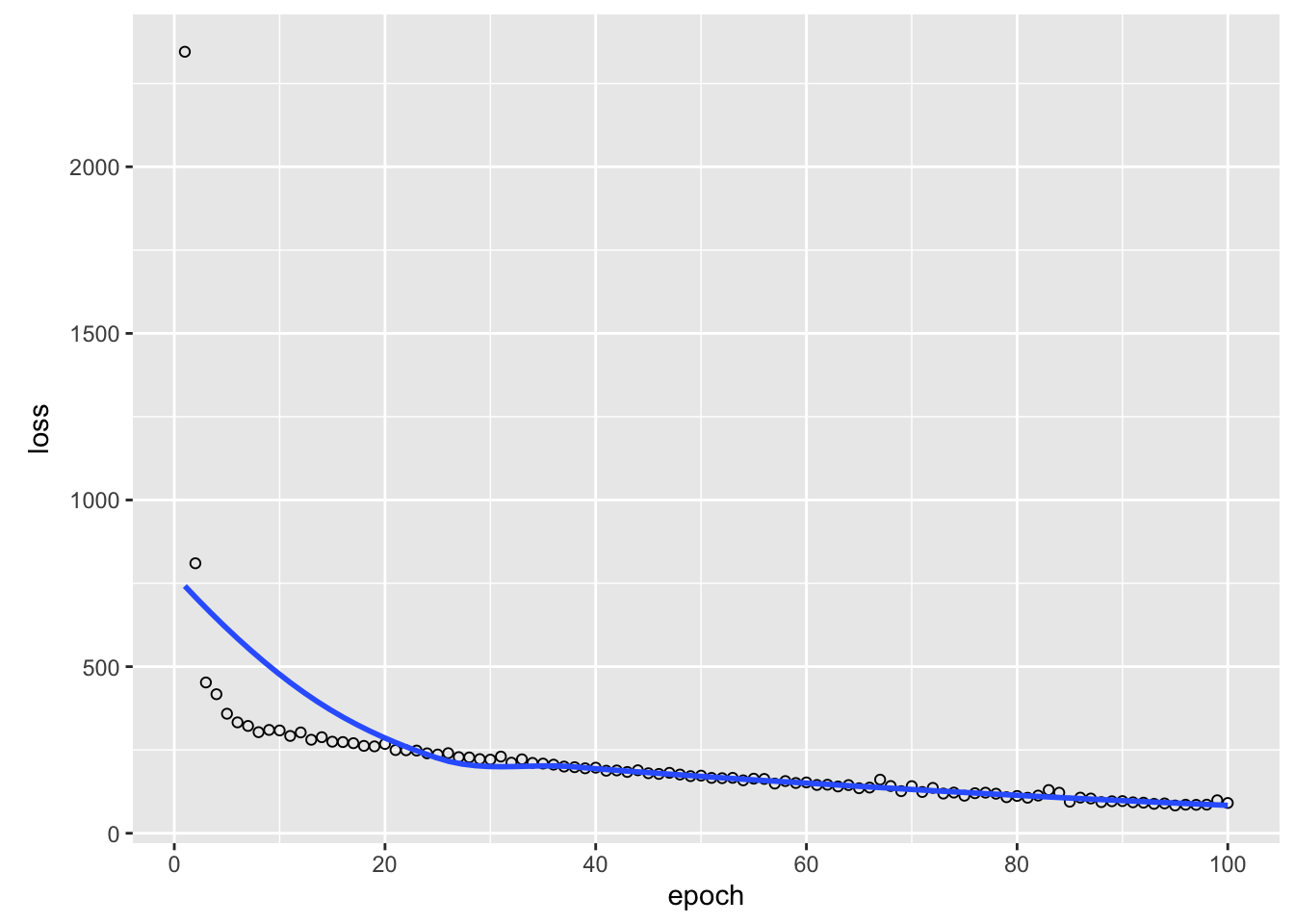
pred_keras = predict(model, x)4/4 - 0s - 5ms/stepfit = lm(Ozone ~ ., data = data)
pred_lm = predict(fit, data)
rmse_lm = mean(sqrt((y - pred_lm)^2))
rmse_keras = mean(sqrt((y - pred_keras)^2))
print(rmse_lm)[1] 14.78897print(rmse_keras)[1] 6.317963Before we start, load and prepare the data set:
library(torch)
data = airquality
summary(data) Ozone Solar.R Wind Temp
Min. : 1.00 Min. : 7.0 Min. : 1.700 Min. :56.00
1st Qu.: 18.00 1st Qu.:115.8 1st Qu.: 7.400 1st Qu.:72.00
Median : 31.50 Median :205.0 Median : 9.700 Median :79.00
Mean : 42.13 Mean :185.9 Mean : 9.958 Mean :77.88
3rd Qu.: 63.25 3rd Qu.:258.8 3rd Qu.:11.500 3rd Qu.:85.00
Max. :168.00 Max. :334.0 Max. :20.700 Max. :97.00
NAs :37 NAs :7
Month Day
Min. :5.000 Min. : 1.0
1st Qu.:6.000 1st Qu.: 8.0
Median :7.000 Median :16.0
Mean :6.993 Mean :15.8
3rd Qu.:8.000 3rd Qu.:23.0
Max. :9.000 Max. :31.0
plot(data)
data = data[complete.cases(data),] # Remove NAs.
summary(data) Ozone Solar.R Wind Temp
Min. : 1.0 Min. : 7.0 Min. : 2.30 Min. :57.00
1st Qu.: 18.0 1st Qu.:113.5 1st Qu.: 7.40 1st Qu.:71.00
Median : 31.0 Median :207.0 Median : 9.70 Median :79.00
Mean : 42.1 Mean :184.8 Mean : 9.94 Mean :77.79
3rd Qu.: 62.0 3rd Qu.:255.5 3rd Qu.:11.50 3rd Qu.:84.50
Max. :168.0 Max. :334.0 Max. :20.70 Max. :97.00
Month Day
Min. :5.000 Min. : 1.00
1st Qu.:6.000 1st Qu.: 9.00
Median :7.000 Median :16.00
Mean :7.216 Mean :15.95
3rd Qu.:9.000 3rd Qu.:22.50
Max. :9.000 Max. :31.00 x = scale(data[,2:6])
y = data[,1]model_torch =
nn_sequential(
nn_linear(5L, 20L),
...
nn_linear(20L, 1L),
)library(torch)
model_torch =
nn_sequential(
nn_linear(5L, 20L),
nn_relu(),
nn_linear(20L, 20L),
nn_relu(),
nn_linear(20L, 20L),
nn_relu(),
nn_linear(20L, 1L),
)We have to pass the network’s parameters to the optimizer (how is this different to keras?)
optimizer_torch = optim_adam(params = model_torch$parameters, lr = 0.05)In torch we write the trainings loop on our own. Complete the trainings loop:
# Calculate number of training steps.
epochs = ...
batch_size = 32
steps = ...
X_torch = torch_tensor(x)
Y_torch = torch_tensor(y, ...)
# Set model into training status.
model_torch$train()
log_losses = NULL
# Training loop.
for(i in 1:steps){
# Get batch indices.
indices = sample.int(nrow(x), batch_size)
X_batch = ...
Y_batch = ...
# Reset backpropagation.
optimizer_torch$zero_grad()
# Predict and calculate loss.
pred = model_torch(X_batch)
loss = ...
# Backpropagation and weight update.
loss$backward()
optimizer_torch$step()
log_losses[i] = as.numeric(loss)
}# Calculate number of training steps.
epochs = 100
batch_size = 32
steps = round(nrow(x)/batch_size*epochs)
X_torch = torch_tensor(x)
Y_torch = torch_tensor(y, dtype = torch_float32())$view(list(-1, 1))
# Set model into training status.
model_torch$train()
log_losses = NULL
# Training loop.
for(i in 1:steps){
# Get batch indices.
indices = sample.int(nrow(x), batch_size)
X_batch = X_torch[indices,]
Y_batch = Y_torch[indices,]
# Reset backpropagation.
optimizer_torch$zero_grad()
# Predict and calculate loss.
pred = model_torch(X_batch)
loss = nnf_mse_loss(pred, Y_batch)
# Backpropagation and weight update.
loss$backward()
optimizer_torch$step()
log_losses[i] = as.numeric(loss)
}Tips:
plot(y = log_losses, x = 1:steps, xlab = "Epoch", ylab = "MSE")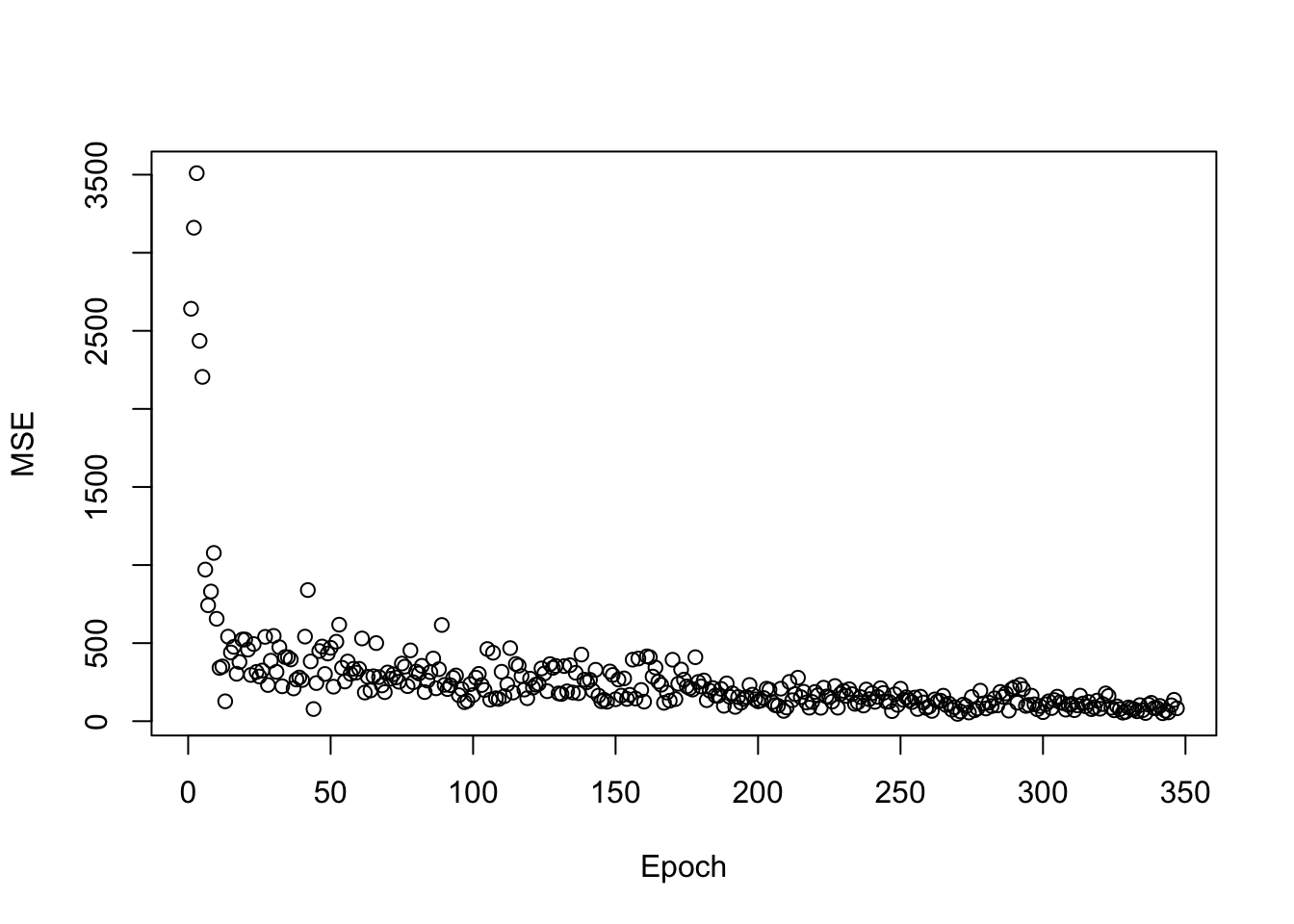
pred_torch = model_torch(X_torch)
pred_torch = as.numeric(pred_torch) # cast torch to R object fit = lm(Ozone ~ ., data = data)
pred_lm = predict(fit, data)
rmse_lm = mean(sqrt((y - pred_lm)^2))
rmse_torch = mean(sqrt((y - pred_torch)^2))
print(rmse_lm)[1] 14.78897print(rmse_torch)[1] 6.897069Build a Keras DNN for the titanic dataset
library(EcoData)
library(dplyr)
Attaching package: 'dplyr'The following objects are masked from 'package:stats':
filter, lagThe following objects are masked from 'package:base':
intersect, setdiff, setequal, unionlibrary(missRanger)
library(torch)
data(titanic_ml)
data = titanic_ml
data =
data |> select(survived, sex, age, fare, pclass)
data[,-1] = missRanger(data[,-1], verbose = 0)
data_sub =
data |>
mutate(age = scales::rescale(age, c(0, 1)),
fare = scales::rescale(fare, c(0, 1))) |>
mutate(sex = as.integer(sex) - 1L,
pclass = as.integer(pclass - 1L))
data_new = data_sub[is.na(data_sub$survived),] # for which we want to make predictions at the end
data_obs = data_sub[!is.na(data_sub$survived),] # data with known response
Xtorch = data_obs[,-1] |> as.matrix() |> torch_tensor()
Ytorch = data_obs[,1] |> as.matrix() |> torch_tensor(dtype=torch_float32())
Xtest = data_new[,-1] |> as.matrix() |> torch_tensor()Dataset:
train_indices = 1:400
val_indices = 401:nrow(Xtorch)
dataset_train= torch::tensor_dataset(Xtorch[train_indices,], Ytorch[train_indices,])
train_dl = torch::dataloader(dataset_train, batch_size = 20L, shuffle = TRUE)
dataset_val= torch::tensor_dataset(Xtorch[val_indices,], Ytorch[val_indices,])
val_dl = torch::dataloader(dataset_val, batch_size = 20L, shuffle = TRUE)
first_batch = train_dl$.iter()
df = first_batch$.next()
df[[1]] |> head()torch_tensor
0.0000 0.2735 0.0151 2.0000
1.0000 0.3444 0.0152 2.0000
1.0000 0.2860 0.0154 2.0000
0.0000 0.2993 0.0282 2.0000
1.0000 0.3236 0.0169 2.0000
1.0000 0.1106 0.0401 2.0000
[ CPUFloatType{6,4} ]df[[2]] |> head()torch_tensor
1
0
0
0
0
1
[ CPUFloatType{6,1} ]Model:
# blueprint
net = nn_module(
# first function tells torch how to build the network
initialize = function(units = 50L, input_dim=4L, dropout_rate = 0.5) {
# self
self$layer1 = nn_linear(in_features = input_dim, out_features = units)
self$dropout1 = nn_dropout(p = dropout_rate)
self$layer2 = nn_linear(units, units)
self$dropout2 = nn_dropout(p = dropout_rate)
self$layer3 = nn_linear(units, 1L)
},
# forward tells torch the input data should be processed
forward = function(x) {
# x = feature tensor
x |>
self$layer1() |>
nnf_relu() |>
self$dropout1() |>
self$layer2() |>
nnf_relu() |>
self$dropout2() |>
self$layer3() |>
torch_sigmoid()
}
)Training loop:
train_dl = torch::dataloader(dataset_train, batch_size = 150L, shuffle = TRUE)
val_dl = torch::dataloader(dataset_val, batch_size = 150L, shuffle = TRUE)
model = net()
opt = optim_adam(params = model$parameters, lr = 0.01)
epochs = 500L
overall_train_loss = overall_val_loss = c()
alpha = 0.7
lambda = 0.01
for(e in 1:epochs) {
losses = losses_val = c()
model$train() # -> dropout is on
coro::loop(
for(batch in train_dl) {
x = batch[[1]] # Feature matrix/tensor
y = batch[[2]] # Response matrix/tensor
opt$zero_grad() # reset optimizer
pred = model(x)
loss = nnf_binary_cross_entropy(pred, y)
# add regularization loss, l2 -> sum((weights)**2)*lambda
loss = loss + (1-alpha)*(lambda*sum(model$parameters[[1]]**2))
# l1 regularization: sum(abs(weights))*lambda
loss = loss + (alpha)*(lambda*sum(abs(model$parameters[[1]])))
loss$backward()
opt$step() # update weights
losses = c(losses, loss$item())
}
)
# calculate validation loss after each epoch
model$eval() # dropout is off
coro::loop(
for(batch in val_dl) {
x = batch[[1]] # Feature matrix/tensor
y = batch[[2]] # Response matrix/tensor
pred = model(x)
loss = nnf_binary_cross_entropy(pred, y)
losses_val = c(losses_val, loss$item())
}
)
overall_train_loss = c(overall_train_loss, mean(losses))
overall_val_loss = c(overall_val_loss, mean(losses_val))
cat(sprintf("Loss at epoch: %d train: %3f eval: %3f\n", e, mean(losses), mean(losses_val)))
}Loss at epoch: 1 train: 1.061287 eval: 0.646822
Loss at epoch: 2 train: 0.973283 eval: 0.652817
Loss at epoch: 3 train: 0.932252 eval: 0.623445
Loss at epoch: 4 train: 0.881706 eval: 0.612755
Loss at epoch: 5 train: 0.838846 eval: 0.601039
Loss at epoch: 6 train: 0.794143 eval: 0.578016
Loss at epoch: 7 train: 0.788708 eval: 0.562789
Loss at epoch: 8 train: 0.717368 eval: 0.540282
Loss at epoch: 9 train: 0.723465 eval: 0.533487
Loss at epoch: 10 train: 0.659200 eval: 0.522329
Loss at epoch: 11 train: 0.664211 eval: 0.522649
Loss at epoch: 12 train: 0.612222 eval: 0.514556
Loss at epoch: 13 train: 0.613024 eval: 0.500222
Loss at epoch: 14 train: 0.607520 eval: 0.487394
Loss at epoch: 15 train: 0.612270 eval: 0.494097
Loss at epoch: 16 train: 0.587178 eval: 0.499945
Loss at epoch: 17 train: 0.554300 eval: 0.482750
Loss at epoch: 18 train: 0.561841 eval: 0.488962
Loss at epoch: 19 train: 0.586277 eval: 0.484681
Loss at epoch: 20 train: 0.559775 eval: 0.480452
Loss at epoch: 21 train: 0.561195 eval: 0.485779
Loss at epoch: 22 train: 0.554978 eval: 0.486634
Loss at epoch: 23 train: 0.566058 eval: 0.491321
Loss at epoch: 24 train: 0.555117 eval: 0.482375
Loss at epoch: 25 train: 0.550732 eval: 0.481965
Loss at epoch: 26 train: 0.532506 eval: 0.478239
Loss at epoch: 27 train: 0.541434 eval: 0.482824
Loss at epoch: 28 train: 0.547886 eval: 0.490667
Loss at epoch: 29 train: 0.543194 eval: 0.479447
Loss at epoch: 30 train: 0.542096 eval: 0.481395
Loss at epoch: 31 train: 0.569523 eval: 0.472467
Loss at epoch: 32 train: 0.520432 eval: 0.482531
Loss at epoch: 33 train: 0.551853 eval: 0.476946
Loss at epoch: 34 train: 0.531947 eval: 0.478664
Loss at epoch: 35 train: 0.526163 eval: 0.485173
Loss at epoch: 36 train: 0.553210 eval: 0.486571
Loss at epoch: 37 train: 0.524824 eval: 0.482460
Loss at epoch: 38 train: 0.527222 eval: 0.471737
Loss at epoch: 39 train: 0.535728 eval: 0.478461
Loss at epoch: 40 train: 0.573437 eval: 0.472048
Loss at epoch: 41 train: 0.510421 eval: 0.482229
Loss at epoch: 42 train: 0.525551 eval: 0.480425
Loss at epoch: 43 train: 0.539331 eval: 0.483444
Loss at epoch: 44 train: 0.524326 eval: 0.480079
Loss at epoch: 45 train: 0.529846 eval: 0.481549
Loss at epoch: 46 train: 0.534244 eval: 0.472180
Loss at epoch: 47 train: 0.522389 eval: 0.473462
Loss at epoch: 48 train: 0.525819 eval: 0.478135
Loss at epoch: 49 train: 0.537413 eval: 0.466751
Loss at epoch: 50 train: 0.544840 eval: 0.459146
Loss at epoch: 51 train: 0.528388 eval: 0.486819
Loss at epoch: 52 train: 0.533555 eval: 0.465963
Loss at epoch: 53 train: 0.546339 eval: 0.476492
Loss at epoch: 54 train: 0.535490 eval: 0.480250
Loss at epoch: 55 train: 0.537781 eval: 0.474570
Loss at epoch: 56 train: 0.522829 eval: 0.473763
Loss at epoch: 57 train: 0.533746 eval: 0.471530
Loss at epoch: 58 train: 0.500943 eval: 0.480092
Loss at epoch: 59 train: 0.550841 eval: 0.465479
Loss at epoch: 60 train: 0.522388 eval: 0.465922
Loss at epoch: 61 train: 0.516799 eval: 0.474731
Loss at epoch: 62 train: 0.523272 eval: 0.474029
Loss at epoch: 63 train: 0.532005 eval: 0.470254
Loss at epoch: 64 train: 0.515423 eval: 0.478724
Loss at epoch: 65 train: 0.511948 eval: 0.474977
Loss at epoch: 66 train: 0.515090 eval: 0.473491
Loss at epoch: 67 train: 0.533681 eval: 0.468289
Loss at epoch: 68 train: 0.517115 eval: 0.479768
Loss at epoch: 69 train: 0.543463 eval: 0.473255
Loss at epoch: 70 train: 0.506904 eval: 0.471708
Loss at epoch: 71 train: 0.515715 eval: 0.467660
Loss at epoch: 72 train: 0.523478 eval: 0.495652
Loss at epoch: 73 train: 0.520893 eval: 0.485845
Loss at epoch: 74 train: 0.533017 eval: 0.473370
Loss at epoch: 75 train: 0.517889 eval: 0.471389
Loss at epoch: 76 train: 0.517371 eval: 0.477436
Loss at epoch: 77 train: 0.540815 eval: 0.468353
Loss at epoch: 78 train: 0.526070 eval: 0.461190
Loss at epoch: 79 train: 0.529169 eval: 0.470275
Loss at epoch: 80 train: 0.507615 eval: 0.476921
Loss at epoch: 81 train: 0.527837 eval: 0.474002
Loss at epoch: 82 train: 0.520113 eval: 0.472925
Loss at epoch: 83 train: 0.513032 eval: 0.463894
Loss at epoch: 84 train: 0.512073 eval: 0.470341
Loss at epoch: 85 train: 0.536100 eval: 0.475027
Loss at epoch: 86 train: 0.518713 eval: 0.476431
Loss at epoch: 87 train: 0.515439 eval: 0.476523
Loss at epoch: 88 train: 0.518799 eval: 0.475238
Loss at epoch: 89 train: 0.509792 eval: 0.470036
Loss at epoch: 90 train: 0.538611 eval: 0.468533
Loss at epoch: 91 train: 0.520385 eval: 0.476044
Loss at epoch: 92 train: 0.552512 eval: 0.473783
Loss at epoch: 93 train: 0.521310 eval: 0.476037
Loss at epoch: 94 train: 0.528451 eval: 0.483846
Loss at epoch: 95 train: 0.504565 eval: 0.486744
Loss at epoch: 96 train: 0.506201 eval: 0.480809
Loss at epoch: 97 train: 0.517127 eval: 0.478596
Loss at epoch: 98 train: 0.520610 eval: 0.478937
Loss at epoch: 99 train: 0.513190 eval: 0.472132
Loss at epoch: 100 train: 0.521543 eval: 0.477064
Loss at epoch: 101 train: 0.542991 eval: 0.469449
Loss at epoch: 102 train: 0.528103 eval: 0.483352
Loss at epoch: 103 train: 0.556345 eval: 0.487392
Loss at epoch: 104 train: 0.525585 eval: 0.481894
Loss at epoch: 105 train: 0.507554 eval: 0.477635
Loss at epoch: 106 train: 0.526854 eval: 0.488782
Loss at epoch: 107 train: 0.512393 eval: 0.473428
Loss at epoch: 108 train: 0.500329 eval: 0.486692
Loss at epoch: 109 train: 0.539327 eval: 0.480352
Loss at epoch: 110 train: 0.502053 eval: 0.479354
Loss at epoch: 111 train: 0.503383 eval: 0.485309
Loss at epoch: 112 train: 0.506590 eval: 0.456416
Loss at epoch: 113 train: 0.513507 eval: 0.471576
Loss at epoch: 114 train: 0.500375 eval: 0.465450
Loss at epoch: 115 train: 0.495769 eval: 0.486544
Loss at epoch: 116 train: 0.529496 eval: 0.465582
Loss at epoch: 117 train: 0.529153 eval: 0.483786
Loss at epoch: 118 train: 0.525349 eval: 0.483837
Loss at epoch: 119 train: 0.524844 eval: 0.485120
Loss at epoch: 120 train: 0.529326 eval: 0.478986
Loss at epoch: 121 train: 0.514256 eval: 0.476671
Loss at epoch: 122 train: 0.532409 eval: 0.471552
Loss at epoch: 123 train: 0.549682 eval: 0.475882
Loss at epoch: 124 train: 0.537724 eval: 0.470775
Loss at epoch: 125 train: 0.532290 eval: 0.478319
Loss at epoch: 126 train: 0.515395 eval: 0.479779
Loss at epoch: 127 train: 0.538957 eval: 0.498512
Loss at epoch: 128 train: 0.519862 eval: 0.474230
Loss at epoch: 129 train: 0.531618 eval: 0.469329
Loss at epoch: 130 train: 0.544438 eval: 0.474695
Loss at epoch: 131 train: 0.515901 eval: 0.485917
Loss at epoch: 132 train: 0.522329 eval: 0.472809
Loss at epoch: 133 train: 0.516902 eval: 0.475261
Loss at epoch: 134 train: 0.525488 eval: 0.478491
Loss at epoch: 135 train: 0.495122 eval: 0.479740
Loss at epoch: 136 train: 0.525601 eval: 0.481157
Loss at epoch: 137 train: 0.533952 eval: 0.477023
Loss at epoch: 138 train: 0.511708 eval: 0.479740
Loss at epoch: 139 train: 0.513322 eval: 0.477410
Loss at epoch: 140 train: 0.523309 eval: 0.476431
Loss at epoch: 141 train: 0.535425 eval: 0.483635
Loss at epoch: 142 train: 0.518885 eval: 0.479784
Loss at epoch: 143 train: 0.515777 eval: 0.473884
Loss at epoch: 144 train: 0.545928 eval: 0.475854
Loss at epoch: 145 train: 0.515615 eval: 0.479400
Loss at epoch: 146 train: 0.523142 eval: 0.477056
Loss at epoch: 147 train: 0.531391 eval: 0.489133
Loss at epoch: 148 train: 0.541234 eval: 0.478018
Loss at epoch: 149 train: 0.515093 eval: 0.481644
Loss at epoch: 150 train: 0.534159 eval: 0.474542
Loss at epoch: 151 train: 0.529139 eval: 0.475298
Loss at epoch: 152 train: 0.526665 eval: 0.480136
Loss at epoch: 153 train: 0.532574 eval: 0.466376
Loss at epoch: 154 train: 0.487992 eval: 0.475270
Loss at epoch: 155 train: 0.537415 eval: 0.479676
Loss at epoch: 156 train: 0.527782 eval: 0.477555
Loss at epoch: 157 train: 0.513758 eval: 0.478965
Loss at epoch: 158 train: 0.523775 eval: 0.471459
Loss at epoch: 159 train: 0.500879 eval: 0.470135
Loss at epoch: 160 train: 0.548872 eval: 0.472939
Loss at epoch: 161 train: 0.526362 eval: 0.475895
Loss at epoch: 162 train: 0.511208 eval: 0.470212
Loss at epoch: 163 train: 0.529025 eval: 0.468295
Loss at epoch: 164 train: 0.524789 eval: 0.482668
Loss at epoch: 165 train: 0.529482 eval: 0.472732
Loss at epoch: 166 train: 0.514301 eval: 0.469538
Loss at epoch: 167 train: 0.525686 eval: 0.480762
Loss at epoch: 168 train: 0.527314 eval: 0.475783
Loss at epoch: 169 train: 0.510569 eval: 0.473204
Loss at epoch: 170 train: 0.520806 eval: 0.464590
Loss at epoch: 171 train: 0.528082 eval: 0.477770
Loss at epoch: 172 train: 0.510214 eval: 0.468734
Loss at epoch: 173 train: 0.523259 eval: 0.477500
Loss at epoch: 174 train: 0.508094 eval: 0.470660
Loss at epoch: 175 train: 0.511994 eval: 0.471968
Loss at epoch: 176 train: 0.498541 eval: 0.467518
Loss at epoch: 177 train: 0.511548 eval: 0.479472
Loss at epoch: 178 train: 0.500741 eval: 0.471070
Loss at epoch: 179 train: 0.525904 eval: 0.478152
Loss at epoch: 180 train: 0.540611 eval: 0.477761
Loss at epoch: 181 train: 0.541401 eval: 0.476630
Loss at epoch: 182 train: 0.502372 eval: 0.471854
Loss at epoch: 183 train: 0.539392 eval: 0.471883
Loss at epoch: 184 train: 0.508677 eval: 0.482836
Loss at epoch: 185 train: 0.521213 eval: 0.473917
Loss at epoch: 186 train: 0.503348 eval: 0.489341
Loss at epoch: 187 train: 0.508416 eval: 0.465929
Loss at epoch: 188 train: 0.514389 eval: 0.469254
Loss at epoch: 189 train: 0.495558 eval: 0.472430
Loss at epoch: 190 train: 0.524242 eval: 0.460994
Loss at epoch: 191 train: 0.533373 eval: 0.474138
Loss at epoch: 192 train: 0.512011 eval: 0.471551
Loss at epoch: 193 train: 0.519609 eval: 0.483742
Loss at epoch: 194 train: 0.502651 eval: 0.479629
Loss at epoch: 195 train: 0.534696 eval: 0.473837
Loss at epoch: 196 train: 0.538492 eval: 0.476177
Loss at epoch: 197 train: 0.519315 eval: 0.478281
Loss at epoch: 198 train: 0.536124 eval: 0.474546
Loss at epoch: 199 train: 0.503554 eval: 0.475096
Loss at epoch: 200 train: 0.511498 eval: 0.472484
Loss at epoch: 201 train: 0.511937 eval: 0.471478
Loss at epoch: 202 train: 0.531837 eval: 0.478301
Loss at epoch: 203 train: 0.528176 eval: 0.467283
Loss at epoch: 204 train: 0.530651 eval: 0.469709
Loss at epoch: 205 train: 0.526469 eval: 0.470500
Loss at epoch: 206 train: 0.543161 eval: 0.475500
Loss at epoch: 207 train: 0.517044 eval: 0.479633
Loss at epoch: 208 train: 0.515614 eval: 0.475840
Loss at epoch: 209 train: 0.509124 eval: 0.477978
Loss at epoch: 210 train: 0.523524 eval: 0.466607
Loss at epoch: 211 train: 0.511380 eval: 0.460721
Loss at epoch: 212 train: 0.517890 eval: 0.457432
Loss at epoch: 213 train: 0.504734 eval: 0.461191
Loss at epoch: 214 train: 0.518254 eval: 0.477686
Loss at epoch: 215 train: 0.508818 eval: 0.468161
Loss at epoch: 216 train: 0.513204 eval: 0.468721
Loss at epoch: 217 train: 0.520195 eval: 0.480618
Loss at epoch: 218 train: 0.506905 eval: 0.476326
Loss at epoch: 219 train: 0.506508 eval: 0.460589
Loss at epoch: 220 train: 0.510053 eval: 0.455492
Loss at epoch: 221 train: 0.516267 eval: 0.471518
Loss at epoch: 222 train: 0.513971 eval: 0.485523
Loss at epoch: 223 train: 0.530749 eval: 0.469554
Loss at epoch: 224 train: 0.509351 eval: 0.477320
Loss at epoch: 225 train: 0.511342 eval: 0.477069
Loss at epoch: 226 train: 0.524018 eval: 0.470267
Loss at epoch: 227 train: 0.550424 eval: 0.473120
Loss at epoch: 228 train: 0.503433 eval: 0.466155
Loss at epoch: 229 train: 0.512986 eval: 0.484537
Loss at epoch: 230 train: 0.549369 eval: 0.479204
Loss at epoch: 231 train: 0.515657 eval: 0.482275
Loss at epoch: 232 train: 0.524579 eval: 0.476466
Loss at epoch: 233 train: 0.519156 eval: 0.480778
Loss at epoch: 234 train: 0.503309 eval: 0.465615
Loss at epoch: 235 train: 0.506810 eval: 0.473072
Loss at epoch: 236 train: 0.505293 eval: 0.469841
Loss at epoch: 237 train: 0.525412 eval: 0.482561
Loss at epoch: 238 train: 0.534675 eval: 0.480504
Loss at epoch: 239 train: 0.524243 eval: 0.484386
Loss at epoch: 240 train: 0.519421 eval: 0.484048
Loss at epoch: 241 train: 0.515823 eval: 0.474394
Loss at epoch: 242 train: 0.516562 eval: 0.477639
Loss at epoch: 243 train: 0.510733 eval: 0.478213
Loss at epoch: 244 train: 0.503600 eval: 0.480220
Loss at epoch: 245 train: 0.532044 eval: 0.467035
Loss at epoch: 246 train: 0.510658 eval: 0.468014
Loss at epoch: 247 train: 0.517972 eval: 0.477927
Loss at epoch: 248 train: 0.522469 eval: 0.478788
Loss at epoch: 249 train: 0.525220 eval: 0.487686
Loss at epoch: 250 train: 0.527013 eval: 0.479130
Loss at epoch: 251 train: 0.528323 eval: 0.475973
Loss at epoch: 252 train: 0.530939 eval: 0.467716
Loss at epoch: 253 train: 0.515805 eval: 0.474608
Loss at epoch: 254 train: 0.509961 eval: 0.480325
Loss at epoch: 255 train: 0.513699 eval: 0.476894
Loss at epoch: 256 train: 0.502379 eval: 0.481129
Loss at epoch: 257 train: 0.529551 eval: 0.476972
Loss at epoch: 258 train: 0.500921 eval: 0.473843
Loss at epoch: 259 train: 0.508131 eval: 0.471771
Loss at epoch: 260 train: 0.497336 eval: 0.472340
Loss at epoch: 261 train: 0.521637 eval: 0.473521
Loss at epoch: 262 train: 0.487709 eval: 0.476102
Loss at epoch: 263 train: 0.523535 eval: 0.473934
Loss at epoch: 264 train: 0.508724 eval: 0.485500
Loss at epoch: 265 train: 0.502699 eval: 0.483857
Loss at epoch: 266 train: 0.518721 eval: 0.471847
Loss at epoch: 267 train: 0.512571 eval: 0.471997
Loss at epoch: 268 train: 0.490275 eval: 0.477381
Loss at epoch: 269 train: 0.516848 eval: 0.467807
Loss at epoch: 270 train: 0.524427 eval: 0.463323
Loss at epoch: 271 train: 0.514383 eval: 0.476072
Loss at epoch: 272 train: 0.540817 eval: 0.482552
Loss at epoch: 273 train: 0.514328 eval: 0.477244
Loss at epoch: 274 train: 0.517317 eval: 0.476928
Loss at epoch: 275 train: 0.531181 eval: 0.471515
Loss at epoch: 276 train: 0.532073 eval: 0.483029
Loss at epoch: 277 train: 0.505782 eval: 0.481627
Loss at epoch: 278 train: 0.513663 eval: 0.475461
Loss at epoch: 279 train: 0.523320 eval: 0.484358
Loss at epoch: 280 train: 0.499192 eval: 0.478119
Loss at epoch: 281 train: 0.512460 eval: 0.467533
Loss at epoch: 282 train: 0.509104 eval: 0.471820
Loss at epoch: 283 train: 0.502510 eval: 0.475175
Loss at epoch: 284 train: 0.508605 eval: 0.472311
Loss at epoch: 285 train: 0.514123 eval: 0.469272
Loss at epoch: 286 train: 0.501304 eval: 0.477695
Loss at epoch: 287 train: 0.518710 eval: 0.464192
Loss at epoch: 288 train: 0.515399 eval: 0.472017
Loss at epoch: 289 train: 0.502455 eval: 0.466244
Loss at epoch: 290 train: 0.496864 eval: 0.467315
Loss at epoch: 291 train: 0.519704 eval: 0.487092
Loss at epoch: 292 train: 0.519911 eval: 0.469312
Loss at epoch: 293 train: 0.538106 eval: 0.479243
Loss at epoch: 294 train: 0.490536 eval: 0.483145
Loss at epoch: 295 train: 0.502872 eval: 0.468161
Loss at epoch: 296 train: 0.504024 eval: 0.476353
Loss at epoch: 297 train: 0.506255 eval: 0.480121
Loss at epoch: 298 train: 0.505431 eval: 0.474386
Loss at epoch: 299 train: 0.504813 eval: 0.484131
Loss at epoch: 300 train: 0.503565 eval: 0.476274
Loss at epoch: 301 train: 0.510889 eval: 0.477768
Loss at epoch: 302 train: 0.508477 eval: 0.477331
Loss at epoch: 303 train: 0.525038 eval: 0.477769
Loss at epoch: 304 train: 0.504952 eval: 0.472575
Loss at epoch: 305 train: 0.523386 eval: 0.479984
Loss at epoch: 306 train: 0.508400 eval: 0.478158
Loss at epoch: 307 train: 0.517463 eval: 0.467139
Loss at epoch: 308 train: 0.528200 eval: 0.463948
Loss at epoch: 309 train: 0.521008 eval: 0.478674
Loss at epoch: 310 train: 0.495604 eval: 0.486210
Loss at epoch: 311 train: 0.500471 eval: 0.473305
Loss at epoch: 312 train: 0.517805 eval: 0.460996
Loss at epoch: 313 train: 0.518790 eval: 0.475819
Loss at epoch: 314 train: 0.501703 eval: 0.474406
Loss at epoch: 315 train: 0.485399 eval: 0.475816
Loss at epoch: 316 train: 0.518349 eval: 0.460355
Loss at epoch: 317 train: 0.512160 eval: 0.466745
Loss at epoch: 318 train: 0.519759 eval: 0.471981
Loss at epoch: 319 train: 0.535186 eval: 0.460937
Loss at epoch: 320 train: 0.494801 eval: 0.477672
Loss at epoch: 321 train: 0.520469 eval: 0.473929
Loss at epoch: 322 train: 0.520619 eval: 0.481180
Loss at epoch: 323 train: 0.510922 eval: 0.476046
Loss at epoch: 324 train: 0.518529 eval: 0.471420
Loss at epoch: 325 train: 0.503383 eval: 0.465534
Loss at epoch: 326 train: 0.527935 eval: 0.479353
Loss at epoch: 327 train: 0.523825 eval: 0.467312
Loss at epoch: 328 train: 0.505603 eval: 0.479437
Loss at epoch: 329 train: 0.501625 eval: 0.478837
Loss at epoch: 330 train: 0.513835 eval: 0.471850
Loss at epoch: 331 train: 0.525275 eval: 0.478710
Loss at epoch: 332 train: 0.496257 eval: 0.476064
Loss at epoch: 333 train: 0.538520 eval: 0.473198
Loss at epoch: 334 train: 0.510984 eval: 0.478703
Loss at epoch: 335 train: 0.517980 eval: 0.469465
Loss at epoch: 336 train: 0.517193 eval: 0.469070
Loss at epoch: 337 train: 0.506403 eval: 0.471323
Loss at epoch: 338 train: 0.496319 eval: 0.471952
Loss at epoch: 339 train: 0.506925 eval: 0.475447
Loss at epoch: 340 train: 0.499264 eval: 0.483092
Loss at epoch: 341 train: 0.507511 eval: 0.455090
Loss at epoch: 342 train: 0.508442 eval: 0.472726
Loss at epoch: 343 train: 0.502474 eval: 0.477400
Loss at epoch: 344 train: 0.514926 eval: 0.479394
Loss at epoch: 345 train: 0.513743 eval: 0.472380
Loss at epoch: 346 train: 0.509662 eval: 0.468073
Loss at epoch: 347 train: 0.521902 eval: 0.465777
Loss at epoch: 348 train: 0.529585 eval: 0.474689
Loss at epoch: 349 train: 0.514988 eval: 0.477527
Loss at epoch: 350 train: 0.516498 eval: 0.470009
Loss at epoch: 351 train: 0.508134 eval: 0.468780
Loss at epoch: 352 train: 0.514881 eval: 0.474098
Loss at epoch: 353 train: 0.520519 eval: 0.467602
Loss at epoch: 354 train: 0.490488 eval: 0.474828
Loss at epoch: 355 train: 0.514379 eval: 0.470948
Loss at epoch: 356 train: 0.506796 eval: 0.476393
Loss at epoch: 357 train: 0.506227 eval: 0.469901
Loss at epoch: 358 train: 0.507227 eval: 0.466749
Loss at epoch: 359 train: 0.485148 eval: 0.472376
Loss at epoch: 360 train: 0.520054 eval: 0.467672
Loss at epoch: 361 train: 0.546853 eval: 0.480188
Loss at epoch: 362 train: 0.496344 eval: 0.477256
Loss at epoch: 363 train: 0.505053 eval: 0.479151
Loss at epoch: 364 train: 0.538462 eval: 0.470025
Loss at epoch: 365 train: 0.505589 eval: 0.465718
Loss at epoch: 366 train: 0.507061 eval: 0.474969
Loss at epoch: 367 train: 0.506313 eval: 0.476936
Loss at epoch: 368 train: 0.524341 eval: 0.464428
Loss at epoch: 369 train: 0.530350 eval: 0.468567
Loss at epoch: 370 train: 0.498768 eval: 0.477846
Loss at epoch: 371 train: 0.526616 eval: 0.465228
Loss at epoch: 372 train: 0.497891 eval: 0.472782
Loss at epoch: 373 train: 0.525339 eval: 0.481577
Loss at epoch: 374 train: 0.507321 eval: 0.481362
Loss at epoch: 375 train: 0.515342 eval: 0.471700
Loss at epoch: 376 train: 0.521832 eval: 0.475076
Loss at epoch: 377 train: 0.509817 eval: 0.470422
Loss at epoch: 378 train: 0.517471 eval: 0.479301
Loss at epoch: 379 train: 0.509605 eval: 0.471687
Loss at epoch: 380 train: 0.498275 eval: 0.472003
Loss at epoch: 381 train: 0.523970 eval: 0.473069
Loss at epoch: 382 train: 0.516649 eval: 0.481613
Loss at epoch: 383 train: 0.514557 eval: 0.481566
Loss at epoch: 384 train: 0.516053 eval: 0.477219
Loss at epoch: 385 train: 0.519658 eval: 0.478508
Loss at epoch: 386 train: 0.522005 eval: 0.470170
Loss at epoch: 387 train: 0.497051 eval: 0.472776
Loss at epoch: 388 train: 0.510730 eval: 0.473959
Loss at epoch: 389 train: 0.504158 eval: 0.475189
Loss at epoch: 390 train: 0.520336 eval: 0.474377
Loss at epoch: 391 train: 0.518448 eval: 0.481263
Loss at epoch: 392 train: 0.502027 eval: 0.480843
Loss at epoch: 393 train: 0.510954 eval: 0.472917
Loss at epoch: 394 train: 0.526083 eval: 0.487496
Loss at epoch: 395 train: 0.512081 eval: 0.488424
Loss at epoch: 396 train: 0.530006 eval: 0.485900
Loss at epoch: 397 train: 0.523105 eval: 0.471185
Loss at epoch: 398 train: 0.525018 eval: 0.462362
Loss at epoch: 399 train: 0.512209 eval: 0.463494
Loss at epoch: 400 train: 0.515195 eval: 0.474969
Loss at epoch: 401 train: 0.502022 eval: 0.468208
Loss at epoch: 402 train: 0.531424 eval: 0.474714
Loss at epoch: 403 train: 0.553018 eval: 0.475594
Loss at epoch: 404 train: 0.529607 eval: 0.487787
Loss at epoch: 405 train: 0.506626 eval: 0.484579
Loss at epoch: 406 train: 0.521344 eval: 0.488432
Loss at epoch: 407 train: 0.532550 eval: 0.482522
Loss at epoch: 408 train: 0.514365 eval: 0.471815
Loss at epoch: 409 train: 0.499597 eval: 0.488428
Loss at epoch: 410 train: 0.512336 eval: 0.470922
Loss at epoch: 411 train: 0.507526 eval: 0.471504
Loss at epoch: 412 train: 0.521590 eval: 0.477798
Loss at epoch: 413 train: 0.483543 eval: 0.473289
Loss at epoch: 414 train: 0.497161 eval: 0.477603
Loss at epoch: 415 train: 0.505566 eval: 0.470803
Loss at epoch: 416 train: 0.494948 eval: 0.470138
Loss at epoch: 417 train: 0.510987 eval: 0.479195
Loss at epoch: 418 train: 0.503284 eval: 0.468012
Loss at epoch: 419 train: 0.512072 eval: 0.472886
Loss at epoch: 420 train: 0.519233 eval: 0.464120
Loss at epoch: 421 train: 0.518350 eval: 0.471993
Loss at epoch: 422 train: 0.498078 eval: 0.469219
Loss at epoch: 423 train: 0.526457 eval: 0.472894
Loss at epoch: 424 train: 0.528673 eval: 0.479130
Loss at epoch: 425 train: 0.523184 eval: 0.478274
Loss at epoch: 426 train: 0.521867 eval: 0.473376
Loss at epoch: 427 train: 0.518926 eval: 0.480358
Loss at epoch: 428 train: 0.497829 eval: 0.478989
Loss at epoch: 429 train: 0.494543 eval: 0.474262
Loss at epoch: 430 train: 0.527538 eval: 0.468123
Loss at epoch: 431 train: 0.522624 eval: 0.469795
Loss at epoch: 432 train: 0.508244 eval: 0.471630
Loss at epoch: 433 train: 0.502272 eval: 0.473637
Loss at epoch: 434 train: 0.503187 eval: 0.464021
Loss at epoch: 435 train: 0.509804 eval: 0.467804
Loss at epoch: 436 train: 0.500676 eval: 0.470794
Loss at epoch: 437 train: 0.485055 eval: 0.473179
Loss at epoch: 438 train: 0.504366 eval: 0.478785
Loss at epoch: 439 train: 0.523417 eval: 0.472895
Loss at epoch: 440 train: 0.530904 eval: 0.467910
Loss at epoch: 441 train: 0.511571 eval: 0.479981
Loss at epoch: 442 train: 0.520959 eval: 0.473096
Loss at epoch: 443 train: 0.523833 eval: 0.479704
Loss at epoch: 444 train: 0.517118 eval: 0.486276
Loss at epoch: 445 train: 0.512361 eval: 0.487281
Loss at epoch: 446 train: 0.521949 eval: 0.478811
Loss at epoch: 447 train: 0.488914 eval: 0.476561
Loss at epoch: 448 train: 0.534302 eval: 0.477986
Loss at epoch: 449 train: 0.514539 eval: 0.481816
Loss at epoch: 450 train: 0.528654 eval: 0.470389
Loss at epoch: 451 train: 0.534299 eval: 0.457609
Loss at epoch: 452 train: 0.514223 eval: 0.478209
Loss at epoch: 453 train: 0.528604 eval: 0.483782
Loss at epoch: 454 train: 0.519513 eval: 0.475026
Loss at epoch: 455 train: 0.512645 eval: 0.478744
Loss at epoch: 456 train: 0.508628 eval: 0.477504
Loss at epoch: 457 train: 0.499922 eval: 0.477763
Loss at epoch: 458 train: 0.510791 eval: 0.464382
Loss at epoch: 459 train: 0.526895 eval: 0.467799
Loss at epoch: 460 train: 0.484194 eval: 0.474601
Loss at epoch: 461 train: 0.509845 eval: 0.476484
Loss at epoch: 462 train: 0.491061 eval: 0.469835
Loss at epoch: 463 train: 0.504380 eval: 0.469853
Loss at epoch: 464 train: 0.493590 eval: 0.475725
Loss at epoch: 465 train: 0.528887 eval: 0.476686
Loss at epoch: 466 train: 0.519810 eval: 0.474631
Loss at epoch: 467 train: 0.494452 eval: 0.466604
Loss at epoch: 468 train: 0.514266 eval: 0.477190
Loss at epoch: 469 train: 0.511016 eval: 0.478259
Loss at epoch: 470 train: 0.524920 eval: 0.471554
Loss at epoch: 471 train: 0.502275 eval: 0.467442
Loss at epoch: 472 train: 0.484630 eval: 0.482822
Loss at epoch: 473 train: 0.527309 eval: 0.471671
Loss at epoch: 474 train: 0.506493 eval: 0.484661
Loss at epoch: 475 train: 0.518805 eval: 0.482189
Loss at epoch: 476 train: 0.502731 eval: 0.470868
Loss at epoch: 477 train: 0.514229 eval: 0.480329
Loss at epoch: 478 train: 0.536573 eval: 0.457654
Loss at epoch: 479 train: 0.511348 eval: 0.467604
Loss at epoch: 480 train: 0.505698 eval: 0.479433
Loss at epoch: 481 train: 0.534767 eval: 0.481740
Loss at epoch: 482 train: 0.527413 eval: 0.472127
Loss at epoch: 483 train: 0.534855 eval: 0.473602
Loss at epoch: 484 train: 0.504592 eval: 0.464408
Loss at epoch: 485 train: 0.506635 eval: 0.469453
Loss at epoch: 486 train: 0.517497 eval: 0.484332
Loss at epoch: 487 train: 0.518464 eval: 0.476367
Loss at epoch: 488 train: 0.515330 eval: 0.479235
Loss at epoch: 489 train: 0.507609 eval: 0.478145
Loss at epoch: 490 train: 0.507875 eval: 0.481723
Loss at epoch: 491 train: 0.506054 eval: 0.474830
Loss at epoch: 492 train: 0.527727 eval: 0.469630
Loss at epoch: 493 train: 0.507301 eval: 0.473889
Loss at epoch: 494 train: 0.518091 eval: 0.463911
Loss at epoch: 495 train: 0.516095 eval: 0.482625
Loss at epoch: 496 train: 0.513880 eval: 0.476892
Loss at epoch: 497 train: 0.508010 eval: 0.473305
Loss at epoch: 498 train: 0.495459 eval: 0.472958
Loss at epoch: 499 train: 0.495860 eval: 0.479942
Loss at epoch: 500 train: 0.528116 eval: 0.472794matplot(cbind(overall_train_loss, overall_val_loss), type = "l", lty = 1, col = c("#2262AA", "#F82211"), xlab = "epoch", ylab = "Loss")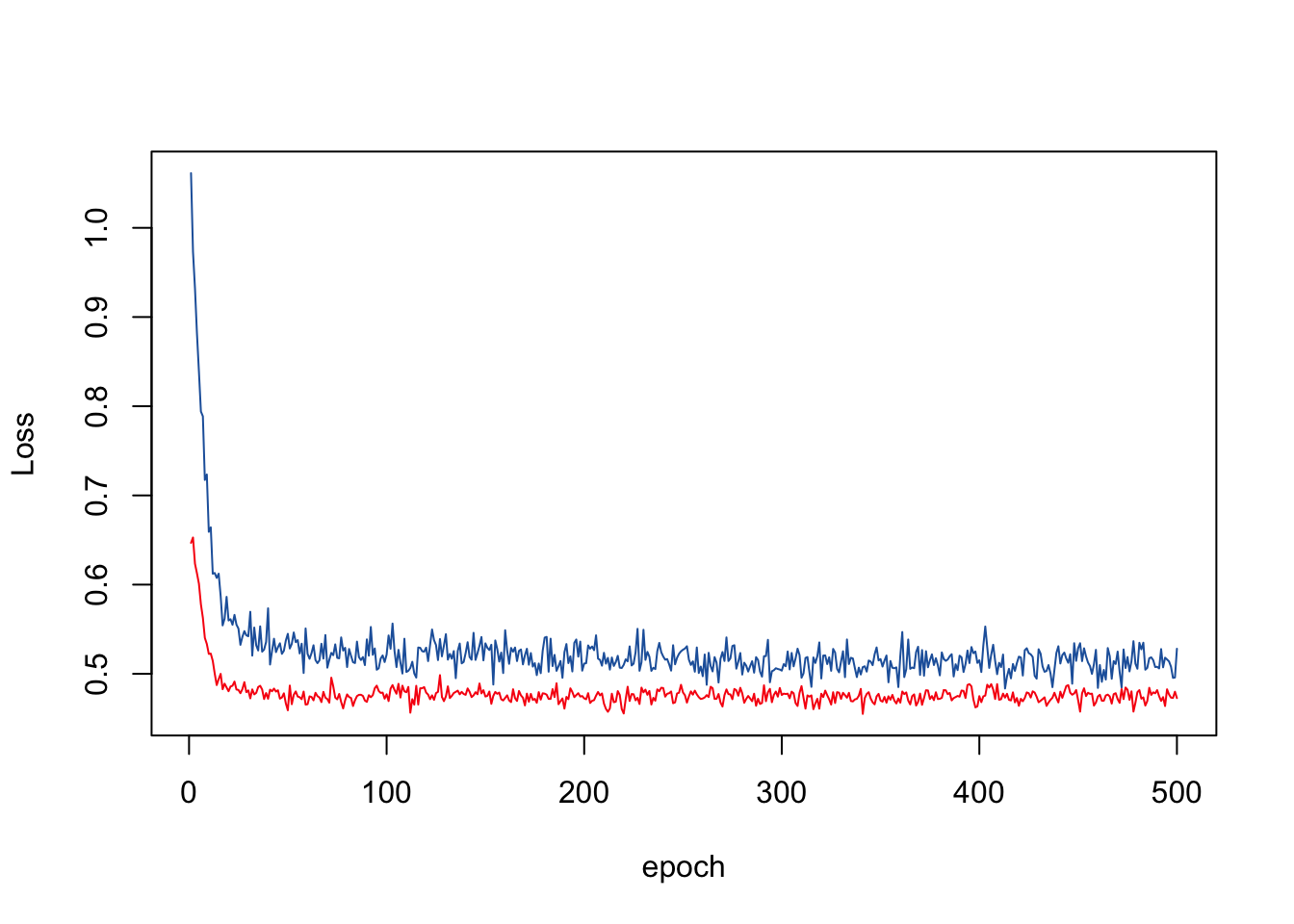
Predictions
model$eval()
predictions = model(Xtest)
predictions = as.numeric(predictions)The next task differs for Torch and Keras users. Keras users will learn more about the inner working of training while Torch users will learn how to simplify and generalize the training loop.
Go through the code and try to understand it.
Similar to Torch, here we will write the training loop ourselves in the following. The training loop consists of several steps:
library(tensorflow)
library(keras3)
data = airquality
data = data[complete.cases(data),] # Remove NAs.
x = scale(data[,2:6])
y = data[,1]
layers = tf$keras$layers
model = tf$keras$models$Sequential(
c(
layers$InputLayer(shape = list(5L)),
layers$Dense(units = 20L, activation = tf$nn$relu),
layers$Dense(units = 20L, activation = tf$nn$relu),
layers$Dense(units = 20L, activation = tf$nn$relu),
layers$Dense(units = 1L, activation = NULL) # No activation == "linear".
)
)
epochs = 200L
optimizer = tf$keras$optimizers$Adamax(0.01)
# Stochastic gradient optimization is more efficient
# in each optimization step, we use a random subset of the data.
get_batch = function(batch_size = 32L){
indices = sample.int(nrow(x), size = batch_size)
return(list(bX = x[indices,], bY = y[indices]))
}
get_batch() # Try out this function.$bX
Solar.R Wind Temp Month Day
79 1.09923936 -1.02302783 0.65133550 -0.1467431 0.235903090
153 0.41905906 0.43858520 -1.02757865 1.2106304 1.614073775
92 0.75914921 -0.20789749 0.33653910 -0.1467431 1.728921332
136 0.58361881 -1.02302783 -0.08318944 1.2106304 -0.338334695
3 -0.39276904 0.74777257 -0.39798584 -1.5041165 -1.486810266
40 1.16506326 1.08506788 1.28092831 -0.8254298 -0.797724924
41 1.51612406 0.43858520 0.96613190 -0.8254298 -0.682877366
151 0.06799826 1.22560759 -0.29305371 1.2106304 1.384378661
31 1.03341546 -0.71384046 -0.18812157 -1.5041165 1.728921332
1 0.05702761 -0.71384046 -1.13251078 -1.5041165 -1.716505380
138 -0.79868308 0.43858520 -0.71278225 1.2106304 -0.108639581
88 -1.12780258 0.57912491 0.86119977 -0.1467431 1.269531104
70 0.95662091 -1.19167548 1.49079258 -0.1467431 -0.797724924
82 -1.95060133 -0.85438017 -0.39798584 -0.1467431 0.580445762
20 -1.54468728 -0.06735777 -1.65717146 -1.5041165 0.465598204
122 0.57264816 -1.02302783 1.91052111 0.5319436 1.614073775
12 0.78109051 -0.06735777 -0.92264652 -1.5041165 -0.453182252
116 0.29838191 -0.06735777 0.12667483 0.5319436 0.924988433
16 1.63680121 0.43858520 -1.44730719 -1.5041165 0.006207976
81 0.38614711 0.43858520 0.75626764 -0.1467431 0.465598204
68 1.00050351 -1.36032314 1.07106404 -0.1467431 -1.027420038
74 -0.10753214 1.39425525 0.33653910 -0.1467431 -0.338334695
147 -1.48983403 0.10128988 -0.92264652 1.2106304 0.924988433
47 0.06799826 1.39425525 -0.08318944 -0.8254298 0.006207976
13 1.15409261 -0.20789749 -1.23744292 -1.5041165 -0.338334695
14 0.97856221 0.26993754 -1.02757865 -1.5041165 -0.223487138
87 -1.13877323 -0.37654514 0.44147123 -0.1467431 1.154683547
100 0.48488296 0.10128988 1.28092831 0.5319436 -0.912572481
38 -0.63412333 -0.06735777 0.44147123 -0.8254298 -1.027420038
133 0.81400246 -0.06735777 -0.50291798 1.2106304 -0.682877366
22 1.48321211 1.87209028 -0.50291798 -1.5041165 0.695293319
111 0.64944271 0.26993754 0.02174269 0.5319436 0.350750647
$bY
[1] 61 20 59 28 12 71 39 14 37 41 13 52 97 16 11 84 16 45 14 63 77 27 7 21 11
[26] 14 20 89 29 24 11 31steps = floor(nrow(x)/32) * epochs # We need nrow(x)/32 steps for each epoch.
for(i in 1:steps){
# Get data.
batch = get_batch()
# Transform it into tensors.
bX = tf$constant(batch$bX)
bY = tf$constant(matrix(batch$bY, ncol = 1L))
# Automatic differentiation:
# Record computations with respect to our model variables.
with(tf$GradientTape() %as% tape,
{
pred = model(bX) # We record the operation for our model weights.
loss = tf$reduce_mean(tf$keras$losses$mse(bY, pred))
}
)
# Calculate the gradients for our model$weights at the loss / backpropagation.
gradients = tape$gradient(loss, model$weights)
# Update our model weights with the learning rate specified above.
optimizer$apply_gradients(purrr::transpose(list(gradients, model$weights)))
if(! i%%30){
cat("Loss: ", loss$numpy(), "\n") # Print loss every 30 steps (not epochs!).
}
}Loss: 1388.129
Loss: 529.437
Loss: 253.1059
Loss: 405.0513
Loss: 265.2523
Loss: 262.1181
Loss: 454.4542
Loss: 214.7283
Loss: 164.4616
Loss: 214.7031
Loss: 210.7287
Loss: 247.4868
Loss: 289.9718
Loss: 201.1375
Loss: 129.5175
Loss: 257.1991
Loss: 197.9713
Loss: 203.05
Loss: 388.7124
Loss: 294.558 Keras and Torch use dataloaders to generate the data batches. Dataloaders are objects that return batches of data infinetly. Keras create the dataloader object automatically in the fit function, in Torch we have to write them ourselves:
library(torch)

data = airquality
data = data[complete.cases(data),]  # Remove NAs.
x = scale(data[,2:6])
y = matrix(data[,1], ncol = 1L)


torch_dataset = torch::dataset(
    name = "airquality",
    initialize = function(X,Y) {
      self$X = torch::torch_tensor(as.matrix(X), dtype = torch_float32())
      self$Y = torch::torch_tensor(as.matrix(Y), dtype = torch_float32())
    },
    .getitem = function(index) {
      x = self$X[index,]
      y = self$Y[index,]
      list(x, y)
    },
    .length = function() {
      self$Y$size()[[1]]
    }
  )
dataset = torch_dataset(x,y)
dataloader = torch::dataloader(dataset, batch_size = 30L, shuffle = TRUE)
Our dataloader is again an object which has to be initiated. The initiated object returns a list of two elements, batch x and batch y. The initated object stops returning batches when the dataset was completly transversed (no worries, we don’t have to all of this ourselves).
Our training loop has changed:
model_torch = nn_sequential(
  nn_linear(5L, 50L),
  nn_relu(),
  nn_linear(50L, 50L),
  nn_relu(),
  nn_linear(50L, 50L),
  nn_relu(),
  nn_linear(50L, 1L)
)
epochs = 50L
opt = optim_adam(model_torch$parameters, 0.01)
train_losses = c()
for(epoch in 1:epochs){
  train_loss = c()
  coro::loop(
    for(batch in dataloader) {
      opt$zero_grad()
      pred = model_torch(batch[[1]])
      loss = nnf_mse_loss(pred, batch[[2]])
      loss$backward()
      opt$step()
      train_loss = c(train_loss, loss$item())
    }
  )
  train_losses = c(train_losses, mean(train_loss))
  if(!epoch%%10) cat(sprintf("Loss at epoch %d: %3f\n", epoch, mean(train_loss)))
}
Loss at epoch 10: 345.274540
Loss at epoch 20: 297.495060
Loss at epoch 30: 262.274254
Loss at epoch 40: 249.399551
Loss at epoch 50: 175.385212plot(train_losses, type = "o", pch = 15,
col = "darkblue", lty = 1, xlab = "Epoch",
ylab = "Loss", las = 1)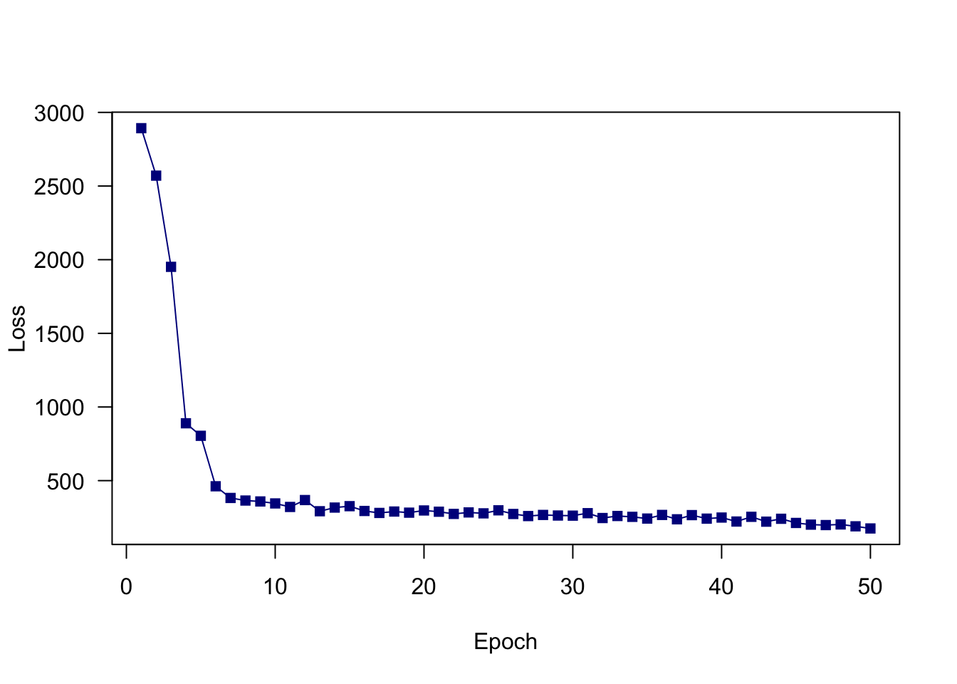
Now change the code from above for the iris data set. Tip: In tf\(keras\)losses$… you can find various loss functions.
library(tensorflow)
library(keras3)

x = scale(iris[,1:4])
y = iris[,5]
y = keras3::to_categorical(as.integer(Y)-1L, 3)

layers = tf$keras$layers
model = tf$keras$models$Sequential(
  c(
    layers$InputLayer(shape = list(4L)),
    layers$Dense(units = 20L, activation = tf$nn$relu),
    layers$Dense(units = 20L, activation = tf$nn$relu),
    layers$Dense(units = 20L, activation = tf$nn$relu),
    layers$Dense(units = 3L, activation = tf$nn$softmax)
  )
)

epochs = 200L
optimizer = tf$keras$optimizers$Adamax(0.01)

# Stochastic gradient optimization is more efficient.
get_batch = function(batch_size = 32L){
  indices = sample.int(nrow(x), size = batch_size)
  return(list(bX = x[indices,], bY = y[indices,]))
}

steps = floor(nrow(x)/32) * epochs # We need nrow(x)/32 steps for each epoch.

for(i in 1:steps){
  batch = get_batch()
  bX = tf$constant(batch$bX)
  bY = tf$constant(batch$bY)

  # Automatic differentiation.
  with(tf$GradientTape() %as% tape,
    {
      pred = model(bX) # we record the operation for our model weights
      loss = tf$reduce_mean(tf$keras$losses$categorical_crossentropy(bY, pred))
    }
  )

  # Calculate the gradients for the loss at our model$weights / backpropagation.
  gradients = tape$gradient(loss, model$weights)

  # Update our model weights with the learning rate specified above.
  optimizer$apply_gradients(purrr::transpose(list(gradients, model$weights)))

  if(! i%%30){
    cat("Loss: ", loss$numpy(), "\n") # Print loss every 30 steps (not epochs!).
  }
}
Loss: 0.002285427
Loss: 0.0004280635
Loss: 0.0004531815
Loss: 0.0002394892
Loss: 0.0007007203
Loss: 0.0003402982
Loss: 0.0002044594
Loss: 0.0001533451
Loss: 0.0001856393
Loss: 0.0001371372
Loss: 0.0001377949
Loss: 0.0001056943
Loss: 0.0001801515
Loss: 0.0001098824
Loss: 5.821453e-05
Loss: 8.931977e-05
Loss: 0.000111592
Loss: 4.739605e-05
Loss: 9.041878e-05
Loss: 5.21631e-05
Loss: 5.589031e-05
Loss: 9.188705e-05
Loss: 5.181757e-05
Loss: 6.043584e-05
Loss: 9.304328e-05
Loss: 4.269042e-05 library(torch)
x = scale(iris[,1:4])
y = iris[,5]
y = as.integer(iris$Species)
torch_dataset = torch::dataset(
name = "iris",
initialize = function(X,Y) {
self$X = torch::torch_tensor(as.matrix(X), dtype = torch_float32())
self$Y = torch::torch_tensor(Y, dtype = torch_long())
},
.getitem = function(index) {
x = self$X[index,]
y = self$Y[index]
list(x, y)
},
.length = function() {
self$Y$size()[[1]]
}
)
dataset = torch_dataset(x,y)
dataloader = torch::dataloader(dataset, batch_size = 30L, shuffle = TRUE)
model_torch = nn_sequential(
nn_linear(4L, 50L),
nn_relu(),
nn_linear(50L, 50L),
nn_relu(),
nn_linear(50L, 50L),
nn_relu(),
nn_linear(50L, 3L)
)
epochs = 50L
opt = optim_adam(model_torch$parameters, 0.01)
train_losses = c()
for(epoch in 1:epochs){
train_loss
coro::loop(
for(batch in dataloader) {
opt$zero_grad()
pred = model_torch(batch[[1]])
loss = nnf_cross_entropy(pred, batch[[2]])
loss$backward()
opt$step()
train_loss = c(train_loss, loss$item())
}
)
train_losses = c(train_losses, mean(train_loss))
if(!epoch%%10) cat(sprintf("Loss at epoch %d: %3f\n", epoch, mean(train_loss)))
}Loss at epoch 10: 13.205854
Loss at epoch 20: 6.885013
Loss at epoch 30: 4.659601
Loss at epoch 40: 3.523018
Loss at epoch 50: 2.833100Remarks:
If are not yet familiar with the underlying concepts of neural networks and want to know more about that, it is suggested to read / view the following videos / sites. Consider the Links and videos with descriptions in parentheses as optional bonus.
This might be useful to understand the further concepts in more depth.
(https://en.wikipedia.org/wiki/Newton%27s_method#Description (Especially the animated graphic is interesting).)
Activation functions in detail (requires the above as prerequisite).
Videos about the topic:
Depending on activation functions, it might occur that the network won’t get updated, even with high learning rates (called vanishing gradient, especially for “sigmoid” functions). Furthermore, updates might overshoot (called exploding gradients) or activation functions will result in many zeros (especially for “relu”, dying relu).
In general, the first layers of a network tend to learn (much) more slowly than subsequent ones.