library(rpart)
library(rpart.plot)

data = airquality[complete.cases(airquality),]5 Tree-based Algorithms
5.1 Classification and Regression Trees
Tree-based algorithms use a series of if-then rules to generate predictions from one or more decision trees. In this lecture, we will explore regression and classification trees using the airquality dataset. There is one important hyperparameter for regression trees: minsplit.
- It controls the depth of tree (see the help of rpart for a description).
- It controls the complexity of the tree and can thus also be seen as a regularization parameter.
Fit and visualize one(!) regression tree:
rt = rpart(Ozone~., data = data, control = rpart.control(minsplit = 10))
rpart.plot(rt)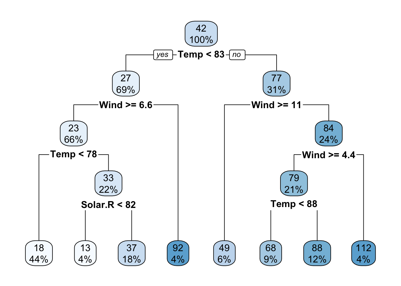
Visualize the predictions:
pred = predict(rt, data)
plot(data$Temp, data$Ozone, xlab = "Temperature", ylab = "Ozone")
lines(data$Temp[order(data$Temp)], pred[order(data$Temp)], col = "red")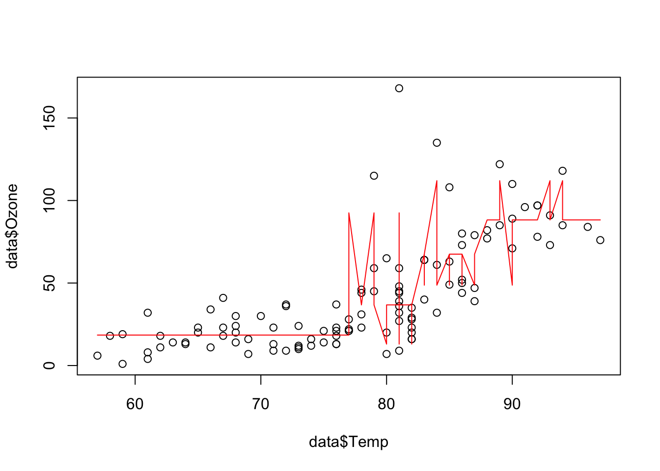
The angular, step-like form of the prediction line is typical for regression trees and is one of their weaknesses.
5.2 Random Forest
To overcome this weakness, a random forest uses an ensemble of regression/classification trees. In principle, a random forest is nothing more than a normal regression/classification tree, but it uses the idea of the “wisdom of the crowd”: by asking many people (the individual trees), you can make a more informed decision (prediction/classification). For example, if you wanted to buy a new phone, you wouldn’t go directly to the store, but you would search the Internet and ask your friends and family.
There are two randomization steps with the random forest that are responsible for their success:
- Bootstrap samples for each tree (we will sample observations with replacement from the data set. For the phone this is like not everyone has experience about each phone).
- At each split, we will sample a subset of predictors that is then considered as potential splitting criterion (for the phone this is like that not everyone has the same decision criteria). Annotation: While building a decision tree (random forests consist of many decision trees), one splits the data at some point according to their features. For example, if you have females and males, tall and short people in a crowd, you can split this crowd by gender and then by size, or by size and then by gender, to build a decision tree.
Applying the random forest follows the same principle as for the methods before: We visualize the data (we have already done this so often for the airquality data set, thus we skip it here), fit the algorithm and then plot the outcomes.
Fit a random forest and visualize the predictions:
library(randomForest)
set.seed(123)

data = airquality[complete.cases(airquality),]

rf = randomForest(Ozone~., data = data)
pred = predict(rf, data)
plot(Ozone~Temp, data = data)
lines(data$Temp[order(data$Temp)], pred[order(data$Temp)], col = "red")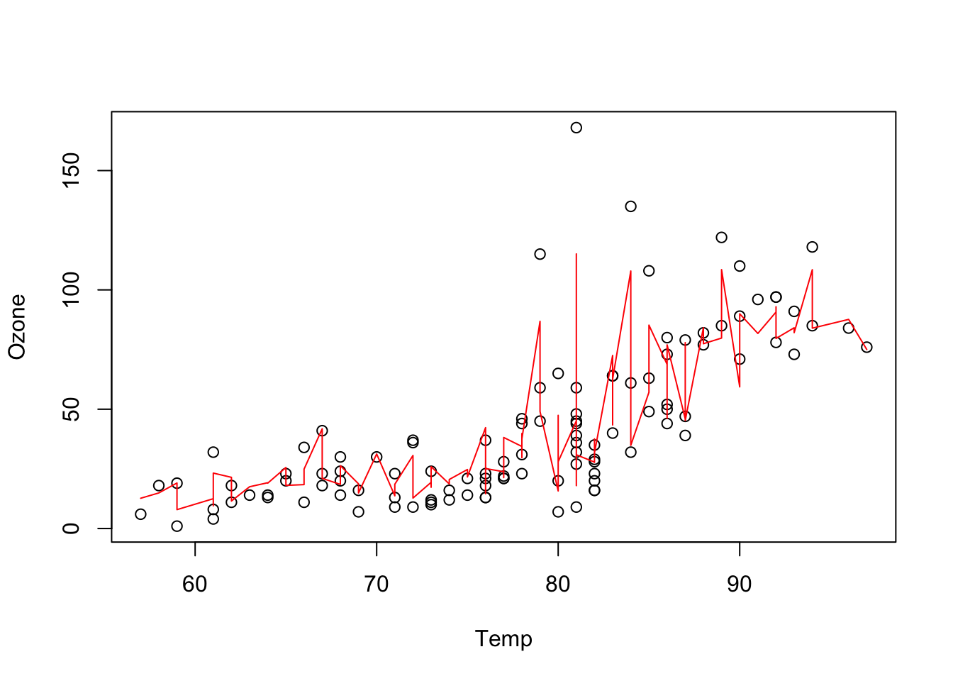
One advantage of random forest is that we get an importance of the variables. For each split in each tree, the improvement in the split criterion is the measure of importance attributed to the split variable, and is accumulated over all trees in the forest separately for each variable. Thus, the variable importance tells us how important a variable is averaged across all trees.
rf$importance IncNodePurity
Solar.R 17467.24
Wind 30691.91
Temp 36076.90
Month 10492.50
Day 15155.45There are several important hyperparameters in a random forest that we can tune to get better results:
| Hyperparameter | Explanation |
|---|---|
| mtry | Subset of features randomly selected in each node (from which the algorithm can select the feature that will be used to split the data). |
| minimum node size | Minimal number of observations allowed in a node (before the branching is canceled) |
| max depth | Maximum number of tree depth |
5.3 Boosted Regression Trees
A boosted regression tree (BRT) starts with a simple regression tree (a weak learner) and then sequentially fits additional trees to improve the results. There are two main strategies:
- AdaBoost: misclassified observations (from the previous tree) get a higher weight, so the next trees focus on the difficult/misclassified observations.
- Gradient boosting (state of the art): each sequential model is fit on the residual errors of the previous model (strongly simplified — the actual algorithm is complex).
We can fit a boosted regression tree using xgboost, but before we have to transform the data into a xgb.Dmatrix (which is a xgboost specific data type, the package sadly doesn’t support R matrices or data.frames).
library(xgboost)
set.seed(123)
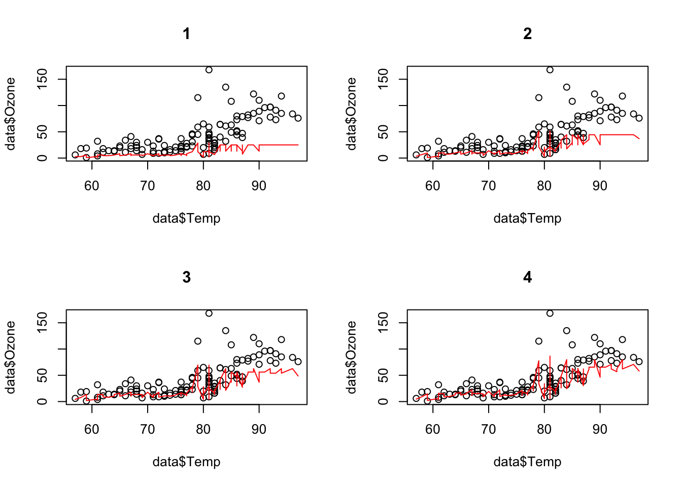
data = airquality[complete.cases(airquality),]brt = xgboost(x= as.matrix(scale(data[,-1])), y = data$Ozone , nrounds = 16L)The parameter “nrounds” controls how many sequential trees we fit, in our example this was 16. When we predict on new data, we can limit the number of trees used to prevent overfitting (remember: each new tree tries to improve the predictions of the previous trees).
Let us visualize the predictions for different numbers of trees:
oldpar = par(mfrow = c(2, 2))
for(i in 1:4){
  pred = predict(brt, newdata = as.matrix(scale(data[,-1])), iteration_range = c(1, i))
  plot(data$Temp, data$Ozone, main = i, xlab = "Temperature", ylab = "Ozone")
  lines(data$Temp[order(data$Temp)], pred[order(data$Temp)], col = "red")
}
par(oldpar)There are also other ways to control for complexity of the boosted regression tree algorithm:
- max_depth: Maximum depth of each tree.
- shrinkage (each tree will get a weight and the weight will decrease with the number of trees).
When having specified the final model, we can obtain the importance of the variables like for random forests:
xgboost::xgb.importance(model = brt) Feature Gain Cover Frequency
<char> <num> <num> <num>
1: Temp 0.584911826 0.30083091 0.24929972
2: Wind 0.341120888 0.33997397 0.22969188
3: Solar.R 0.047530216 0.21343478 0.31932773
4: Day 0.024926924 0.12153369 0.16526611
5: Month 0.001510146 0.02422665 0.03641457sqrt(mean((data$Ozone - pred)^2)) # RMSE[1] 12.67886data_xg = xgb.DMatrix(data = as.matrix(scale(data[,-1])), label = data$Ozone)One important strength of xgboost is that we can directly do a cross-validation (which is independent of the boosted regression tree itself!) and specify its properties with the parameter “n-fold”:
set.seed(123)

brt = xgboost(x = as.matrix(scale(data[,-1])), y = data$Ozone, nrounds = 5L)
brt_cv = xgboost::xgb.cv(data = data_xg, nfold = 3L,
                         nrounds = 3L)
[1] train-rmse:25.289018±2.568153 test-rmse:28.068080±6.838605
[2] train-rmse:19.673719±2.072596 test-rmse:25.496888±8.002477
[3] train-rmse:15.601778±1.624033 test-rmse:23.519734±7.838301 print(brt_cv)##### xgb.cv 3-folds
iter train_rmse_mean train_rmse_std test_rmse_mean test_rmse_std
<int> <num> <num> <num> <num>
1 25.28902 2.568153 28.06808 6.838605
2 19.67372 2.072596 25.49689 8.002477
3 15.60178 1.624033 23.51973 7.838301Annotation: The original data set is randomly partitioned into \(n\) equal sized subsamples. Each time, the model is trained on \(n - 1\) subsets (training set) and tested on the left out set (test set) to judge the performance.
If we do three-folded cross-validation, we actually fit three different boosted regression tree models (xgboost models) on \(\approx 67\%\) of the data points. Afterwards, we judge the performance on the respective holdout. This now tells us how well the model performed.
Important hyperparameters:
| Hyperparameter | Explanation |
|---|---|
| eta | learning rate (weighting of the sequential trees) |
| max depth | maximal depth in the trees (small = low complexity, large = high complexity) |
| subsample | subsample ratio of the data (bootstrap ratio) |
| lambda | regularization strength of the individual trees |
| max tree | maximal number of trees in the ensemble |
5.4 Exercise - Trees
The exercises come in two parts. The first three explore how complexity behaves for each method — a single regression tree, a random forest, and a boosted regression tree — by sweeping the hyperparameter that controls model complexity and watching the predictions change. The remaining exercises then tune and submit models on the titanic and plant-pollinator data.
5.4.0.1 Understanding complexity in Regression Trees
The goal of this exercise is to understand how the hyperparameter mincut (minsplit) affects the complexity of regression trees.
library(tree)
set.seed(123)

data = airquality
rt = tree(Ozone~., data = data,
          control = tree.control(mincut = 1L, nobs = nrow(data)))

plot(rt)
text(rt)
pred = predict(rt, data)
plot(data$Temp, data$Ozone)
lines(data$Temp[order(data$Temp)], pred[order(data$Temp)], col = "red")
sqrt(mean((data$Ozone - pred)^2)) # RMSE
Tasks:
- The code snippet above returns NA for the RMSE, what is wrong in the snippet?
- Read the
tree.controldocumentation, what does the mincut parameter do? - Try different mincut values and check how the predictions (and the RMSE) change. What was wrong in the snippet above?
You should observe: as mincut grows the tree gets coarser — the step function has fewer, wider steps, the training RMSE rises, and the predictions flatten out (more bias, less variance).
Quick check — a very small mincut produces a tree that:
library(tree)
set.seed(123)

data = airquality[complete.cases(airquality),]

doTask = function(mincut){
  rt = tree(Ozone~., data = data,
            control = tree.control(mincut = mincut, nobs = nrow(data)))

  pred = predict(rt, data)
  plot(data$Temp, data$Ozone,
       main = paste0(
         "mincut: ", mincut,
         "\nRMSE: ", round(sqrt(mean((data$Ozone - pred)^2)), 2)
      )
  )
  lines(data$Temp[order(data$Temp)], pred[order(data$Temp)], col = "red")
}

for(i in c(1, 2, 3, 5, 10, 15, 25, 50, 54, 55, 56, 57, 75, 100)){ doTask(i) }

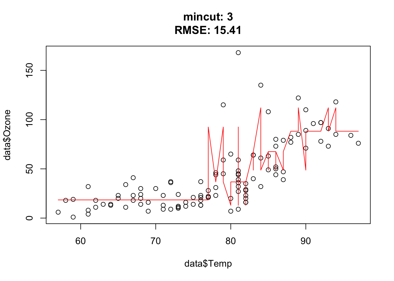

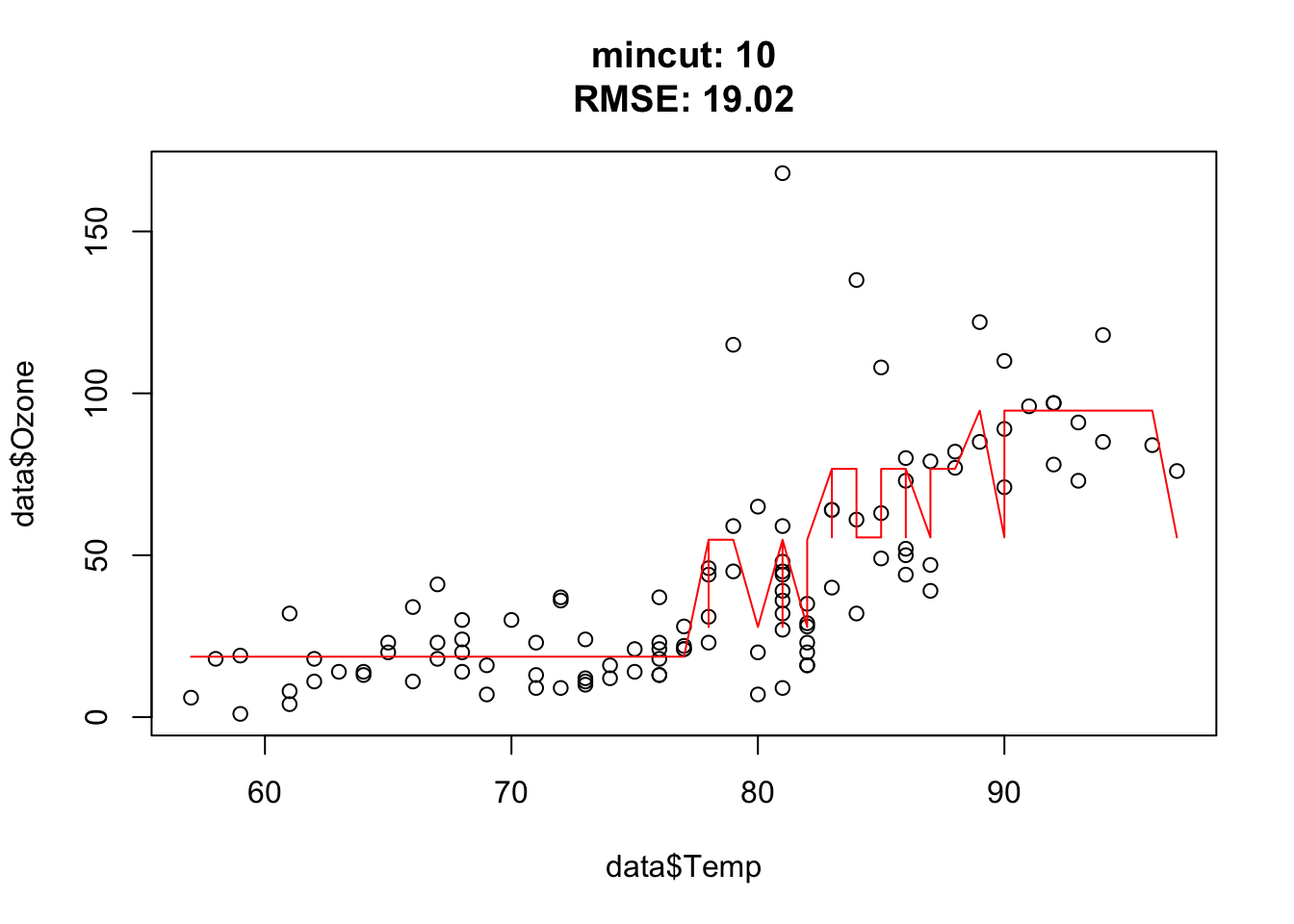


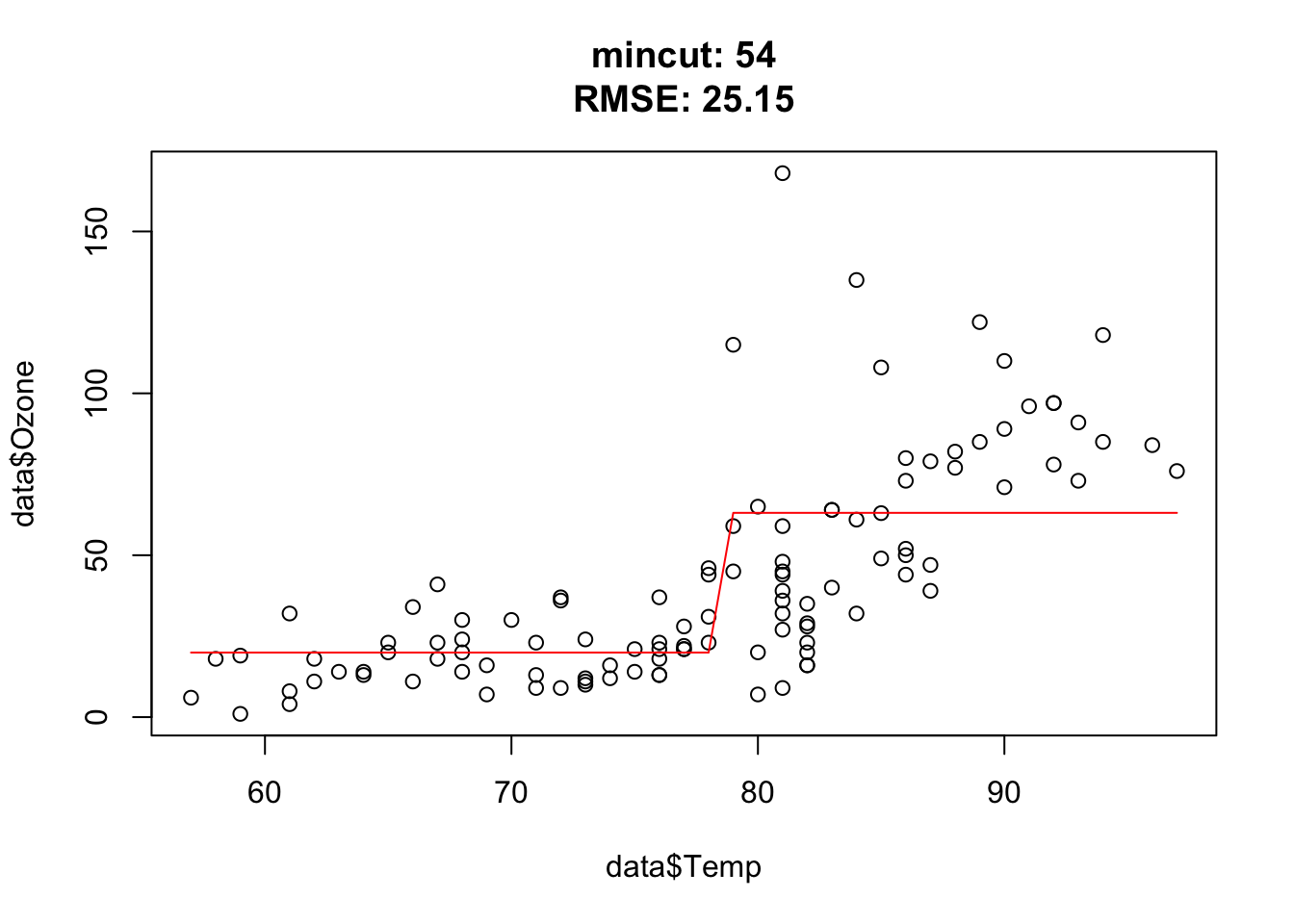

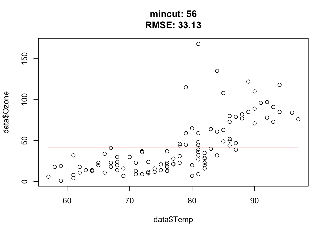


Approximately at mincut = 15, prediction is the best (mind overfitting). After mincut = 56, the prediction has no information at all and the RMSE stays constant.
Mind the complete cases of the airquality data set, that was the error.
5.4.0.2 Understanding complexity in Random forest
The goal of this exercise is to understand how the hyperparameter nodesize affects the complexity of random forest.
library(randomForest)
set.seed(123)

data = airquality[complete.cases(airquality),]

rf = randomForest(Ozone~., data = data)

pred = predict(rf, data)
importance(rf)
IncNodePurity
Solar.R 17467.24
Wind 30691.91
Temp 36076.90
Month 10492.50
Day 15155.45cat("RMSE: ", sqrt(mean((data$Ozone - pred)^2)), "\n")RMSE: 9.63744 plot(data$Temp, data$Ozone)
lines(data$Temp[order(data$Temp)], pred[order(data$Temp)], col = "red")
Tasks:
- Check the documentation of the
randomForestfunction and read the description of the nodesize parameter - Try different nodesize values and describe how the predictions change
You should observe: larger nodesize forces each tree to stop splitting earlier, so the forest becomes smoother and more biased; very small nodesize lets the trees grow deep and fit noise.
Quick check — increasing nodesize makes the random forest:
library(randomForest)
set.seed(123)

data = airquality[complete.cases(airquality),]


for(nodesize in c(1, 15, 50, 100)){
  for(mtry in c(1, 3, 5)){
    rf = randomForest(Ozone~., data = data, nodesize = nodesize, mtry = mtry)

    pred = predict(rf, data)

    plot(data$Temp, data$Ozone, main = paste0(
        "    nodesize: ", nodesize, "    mtry: ", mtry,
        "\nRMSE: ", round(sqrt(mean((data$Ozone - pred)^2)), 2)
      )
    )
    lines(data$Temp[order(data$Temp)], pred[order(data$Temp)], col = "red")
  }
}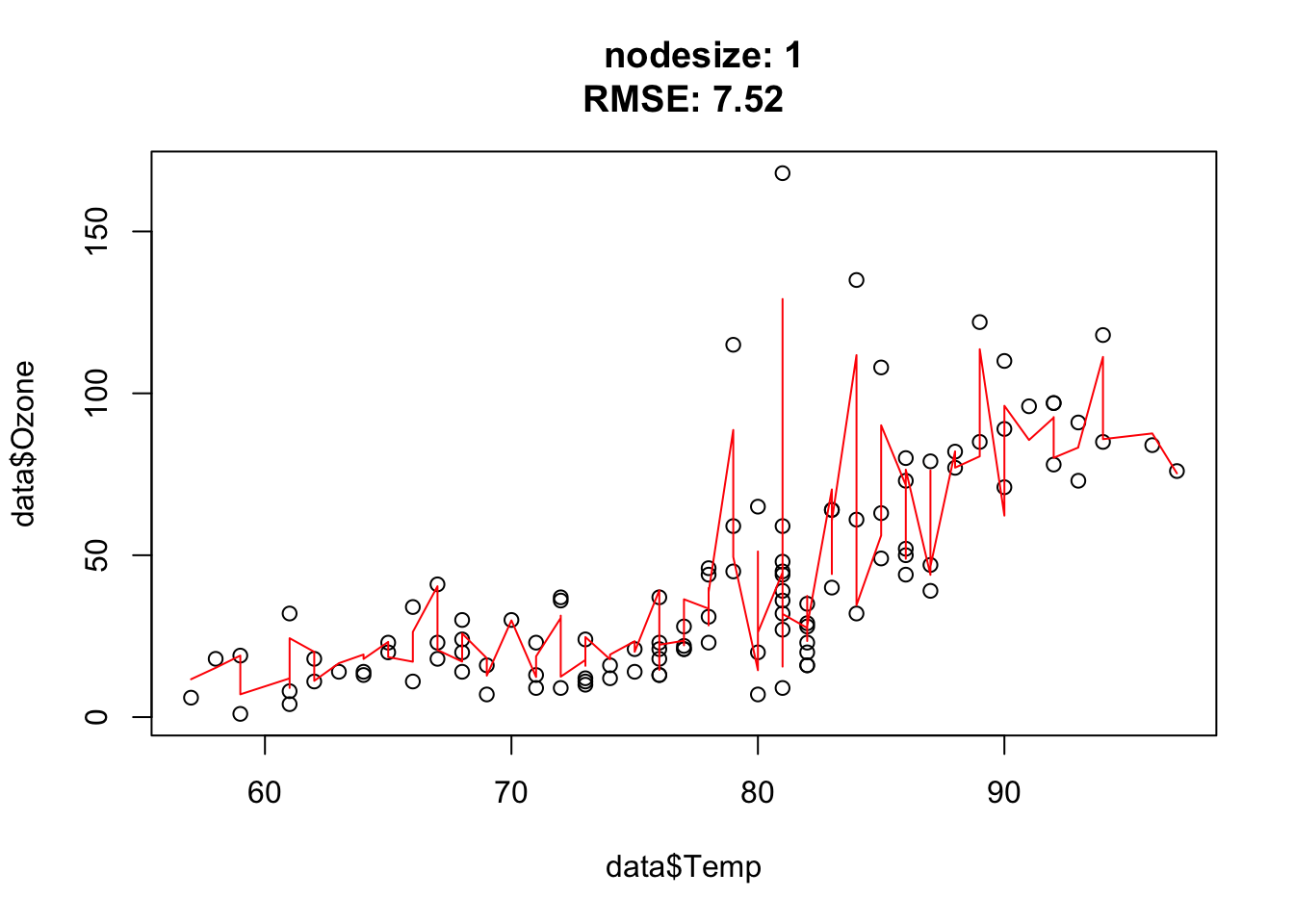


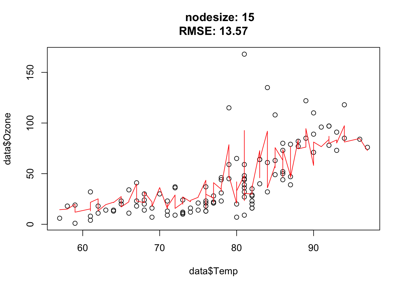
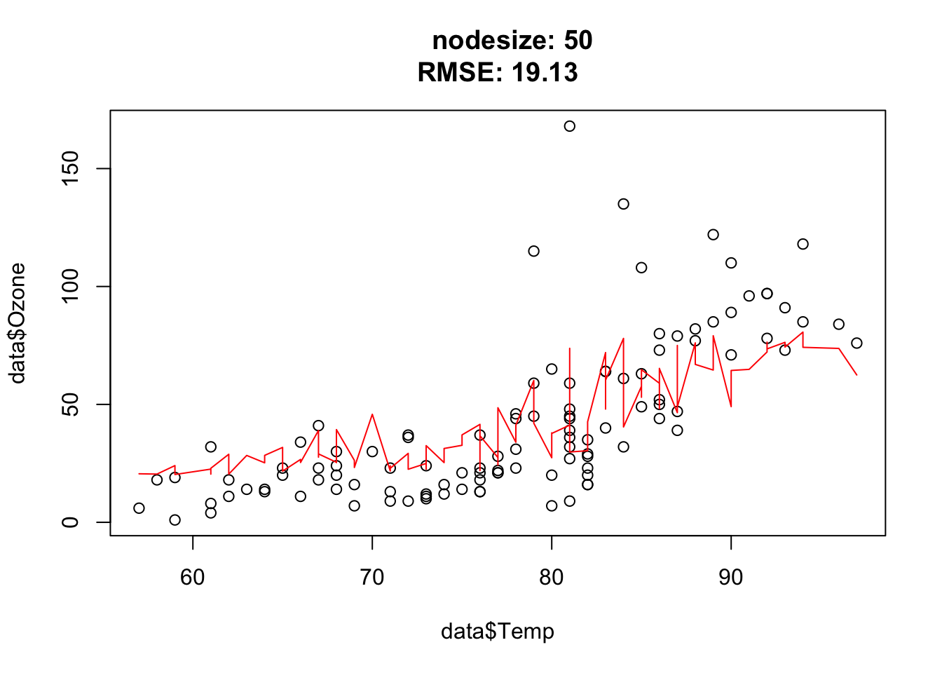


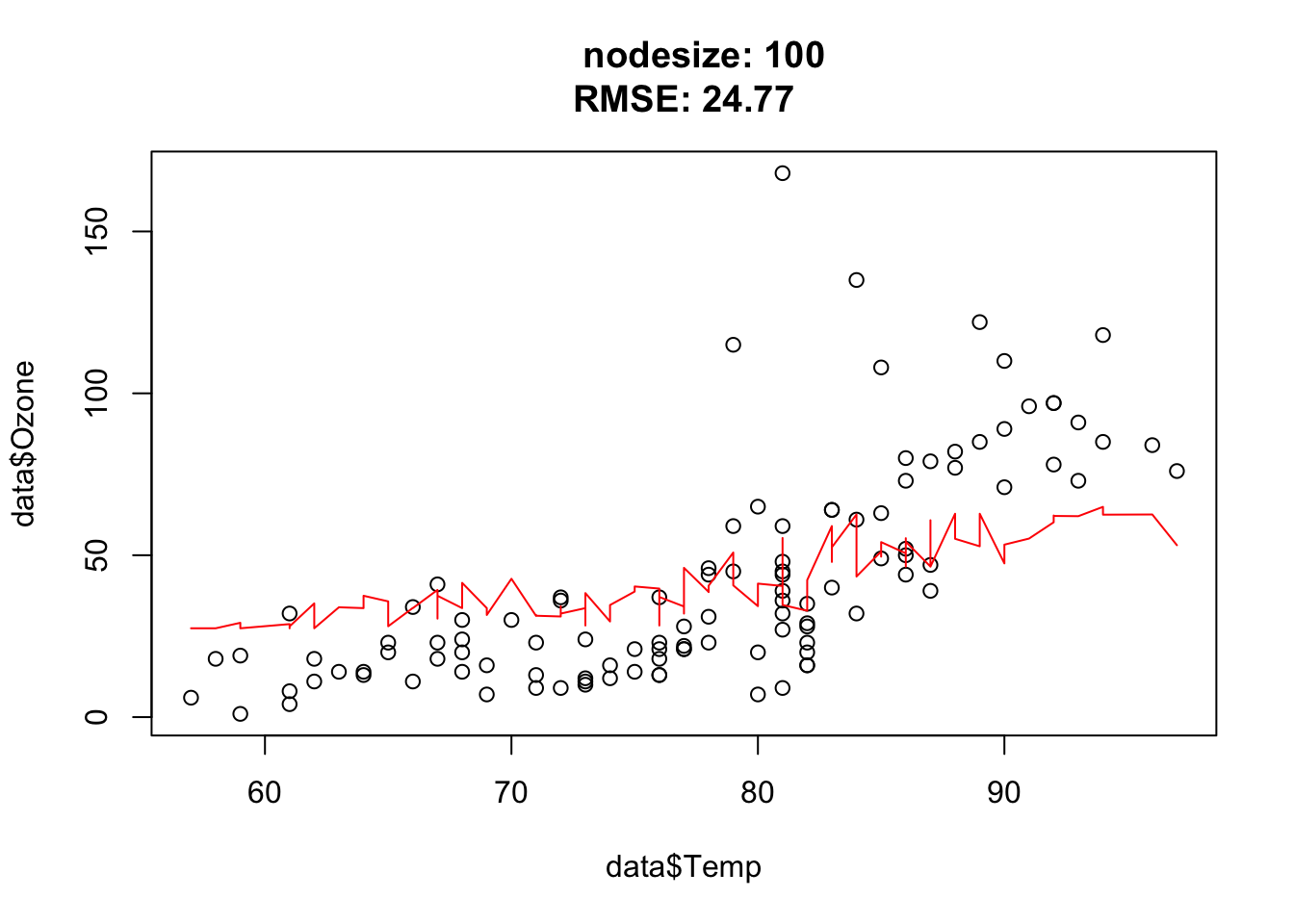
Nodesize affects the complexity. In other words: The bigger the nodesize, the smaller the trees and the more bias/less variance.
5.4.0.3 Understanding complexity in Boosted regression trees
The goal of this exercise is to understand how complexity in BRT affects predictions. For that, we will simulate data with two predictors x1 and x2 and the y response variable will be an interaction of the two predictors:
\[y = e^{-x_1^2 - x_2^2} \] We can visualize the simulated data as an image (x1 and x2 on the x and y axis, and the y values as colors)
library(xgboost)
library(animation)
set.seed(123)

x1 = seq(-3, 3, length.out = 100)
x2 = seq(-3, 3, length.out = 100)
x = expand.grid(x1, x2)
y = apply(x, 1, function(t) exp(-t[1]^2 - t[2]^2))


image(matrix(y, 100, 100), main = "Original image", axes = FALSE, las = 2)
axis(1, at = seq(0, 1, length.out = 10),
     labels = round(seq(-3, 3, length.out = 10), 1))
axis(2, at = seq(0, 1, length.out = 10),
     labels = round(seq(-3, 3, length.out = 10), 1), las = 2)
model = xgboost::xgboost(x = as.matrix(x), y = y,
nrounds = 500L)
pred = predict(model, newdata = as.matrix(x),
iteration_range = c(1, 10L))
saveGIF(
{
for(i in c(1, 2, 4, 8, 12, 20, 40, 80, 200)){
pred = predict(model, newdata = as.matrix(x),
iteration_range = c(1, i))
image(matrix(pred, 100, 100), main = paste0("Trees: ", i),
axes = FALSE, las = 2)
axis(1, at = seq(0, 1, length.out = 10),
labels = round(seq(-3, 3, length.out = 10), 1))
axis(2, at = seq(0, 1, length.out = 10),
labels = round(seq(-3, 3, length.out = 10), 1), las = 2)
}
},
movie.name = "boosting.gif", autobrowse = FALSE
)
Tasks:
- Run the code above and try different max_depth values and describe what you see!
Tip: have a look at the boosting.gif.
You should observe: with a small max_depth each tree is a weak learner, so many boosting rounds are needed before the surface looks smooth; with a large max_depth the fit smooths out after only a few trees (but risks overfitting).
Quick check — with a small max_depth, reaching a smooth fit requires:
library(xgboost)
library(animation)
set.seed(123)

x1 = seq(-3, 3, length.out = 100)
x2 = seq(-3, 3, length.out = 100)
x = expand.grid(x1, x2)
y = apply(x, 1, function(t) exp(-t[1]^2 - t[2]^2))

image(matrix(y, 100, 100), main = "Original image", axes = FALSE, las = 2)
axis(1, at = seq(0, 1, length.out = 10),
     labels = round(seq(-3, 3, length.out = 10), 1))
axis(2, at = seq(0, 1, length.out = 10),
     labels = round(seq(-3, 3, length.out = 10), 1), las = 2)

for(max_depth in c(3, 6, 10, 20)){
  model = xgboost::xgboost(x = as.matrix(x), y = y,
                           max_depth = max_depth,
                           nrounds = 500)

  saveGIF(
    {
      for(i in c(1, 2, 4, 8, 12, 20, 40, 80, 200)){
        pred = predict(model, newdata = as.matrix(x),
                       iteration_range = c(1, i))
        image(matrix(pred, 100, 100),
              main = paste0("max_depth: ", max_depth,
                            "    Trees: ", i),
              axes = FALSE, las = 2)
        axis(1, at = seq(0, 1, length.out = 10),
             labels = round(seq(-3, 3, length.out = 10), 1))
        axis(2, at = seq(0, 1, length.out = 10),
             labels = round(seq(-3, 3, length.out = 10), 1), las = 2)
      }
    },
    movie.name = paste0("boosting_", max_depth, ".gif"),
    autobrowse = FALSE
  )
}
We see that for high values of max_depth, the predictions “smooth out” faster. On the other hand, with a low max_depth (low complexity of the individual trees), more trees are required in the ensemble to achieve a smooth prediction surface.
?xgboost::xgboostJust some examples:

5.4.0.4 Hyperparameter tuning of boosted regression trees
Important hyperparameters:
| Hyperparameter | Explanation |
|---|---|
| eta | learning rate (weighting of the sequential trees) |
| max depth | maximal depth in the trees (small = low complexity, large = high complexity) |
| subsample | subsample ratio of the data (bootstrap ratio) |
| lambda | regularization strength of the individual trees |
| max tree | maximal number of trees in the ensemble |
The goal of this exercise is to tune a BRT on the titanic_ml dataset and beat yesterday’s RF predictions.
Prepare the data:
library(EcoData)
library(dplyr)
Attaching package: 'dplyr'The following object is masked from 'package:randomForest':
combineThe following objects are masked from 'package:stats':
filter, lagThe following objects are masked from 'package:base':
intersect, setdiff, setequal, unionlibrary(missRanger)
data(titanic_ml)
data = titanic_ml
data =
data |> select(survived, sex, age, fare, pclass)
data[,-1] = missRanger(data[,-1], verbose = 0)
data_sub =
data |>
mutate(age = scales::rescale(age, c(0, 1)),
fare = scales::rescale(fare, c(0, 1))) |>
mutate(sex = as.integer(sex) - 1L,
pclass = as.integer(pclass - 1L))
data_new = data_sub[is.na(data_sub$survived),] # for which we want to make predictions at the end
data_obs = data_sub[!is.na(data_sub$survived),] # data with known responseTasks:
- Tune
etaandmax_depthvia cross-validation, then submit your predictions and compare your AUC to yesterday’s random forest. - Interpret: which of the two hyperparameters mattered more for your cross-validated AUC, and how does that map onto the bias-variance tradeoff?
Quick check — we select hyperparameters by the cross-validated AUC rather than the training AUC because:
library(xgboost)
set.seed(42)
data_obs = data_sub[!is.na(data_sub$survived),]
cv = 3
split = sample.int(cv, nrow(data_obs), replace = T)
# sample minnodesize values (must be integers)
hyper_depth = sample(2:10, 20, replace = TRUE)
hyper_eta = runif(20, 0, 1)
tuning_results =
sapply(1:length(hyper_depth), function(k) {
auc_inner = NULL
for(j in 1:cv) {
inner_split = split == j
train_inner = data_obs[!inner_split, ]
test_inner = data_obs[inner_split, ]
data_xg = xgb.DMatrix(data = as.matrix(train_inner[,-1]), label = train_inner$survived)
model = xgb.train(data = data_xg,
nrounds = 16L,
xgb.params(
eta = hyper_eta[k],
max_depth = hyper_depth[k],
objective = "reg:logistic"))
predictions = predict(model, newdata = as.matrix(test_inner[,-1]))
auc_inner[j]= Metrics::auc(test_inner$survived, predictions)
}
return(mean(auc_inner))
})
results = data.frame(depth = hyper_depth, eta = hyper_eta, AUC = tuning_results)
print(results) depth eta AUC
1 4 0.92533996 0.8202916
2 6 0.57483934 0.8049049
3 2 0.91275158 0.8361786
4 3 0.75530192 0.8326217
5 5 0.63099992 0.8263257
6 8 0.79442065 0.8118904
7 2 0.92354646 0.8360385
8 5 0.16446881 0.8170554
9 4 0.19288394 0.8181299
10 2 0.09764267 0.8166034
11 2 0.82910940 0.8341741
12 5 0.80586396 0.8238113
13 10 0.27926999 0.8145355
14 3 0.44902958 0.8318698
15 10 0.62587871 0.8099457
16 6 0.37092142 0.8212375
17 9 0.38231895 0.8147488
18 4 0.91448088 0.8315798
19 3 0.39029775 0.8380767
20 8 0.07029376 0.8100687Make predictions:
data_xg = xgb.DMatrix(data = as.matrix(data_obs[,-1]), label = data_obs$survived)
model = xgb.train(data = data_xg, nrounds = 16L, params = xgb.params(eta = results[which.max(results$AUC), 2], max_depth = results[which.max(results$AUC), 1], objective = "reg:logistic"))
predictions = predict(model, newdata = as.matrix(data_new[,-1]))
# Single predictions from the ensemble model:
write.csv(data.frame(y = predictions), file = "Max_titanic_xgboost.csv")5.4.0.5 Bonus: Walk through a from-scratch BRT
A boosted regression tree is simpler than it looks: fit a weak model, compute the residuals, fit the next model to those residuals, and add it (down-weighted by eta) to the running prediction. Below is a complete, minimal implementation in base R that uses either a small tree or an lm as the weak learner. Your task here is to read and understand it, not to write it from scratch.
As you read, answer for yourself:
- Where are the residuals computed, and which model is fit to them?
- What does the first iteration (
i == 1) do differently from all later iterations? - What role does
etaplay, and what happens to the ensemble asetagets smaller?
library(tree)
#### Helper function for single tree fit.
get_model_tree = function(x, y, ...){
control = tree.control(nobs = length(x), ...)
model = tree(y~., data.frame(x = x, y = y), control = control)
pred = predict(model, newdata = data.frame(x = x, y = y))
return(list(model = model, pred = pred))
}
#### Helper function for single linear model fit.
get_model_linear = function(x, y, ...){
data = data.frame(x = x, y = y)
models = lapply(paste0("y~", colnames(data.frame(x = x))), function(f) lm(as.formula(f), data = data))
model = models[[which.max(abs(sapply(models, coef)[2,]))]]
pred = predict(model, newdata = data.frame(x = x, y = y))
return(list(model = model, pred = pred))
}
#### Boost function.
get_boosting_model = function(x, y, n_trees, bootstrap = NULL, colsample = NULL, eta = 1., booster = "tree", ...){
pred = NULL
m_list = list()
if(booster == "tree") get_model = get_model_tree
else get_model = get_model_linear
for(i in 1:n_trees){
if(i == 1){
m = get_model(x, y, ...)
pred = m$pred
}else{
if(!is.null(bootstrap)) indices = sample.int(length(y), bootstrap*length(y), replace = TRUE)
else indices = 1:length(y)
if(!is.null(colsample)) indices_cols = sample.int(ncol(x), colsample*ncol(x), replace = FALSE)
else indices_cols = 1:ncol(x)
y_res = y[indices] - pred[indices]
m = get_model(x[indices,indices_cols,drop=FALSE], y_res, ...)
pred = pred + eta*predict(m$model, newdata = data.frame(x = x))
}
m_list[[i]] = m$model
}
model_list = list()
model_list$model = m_list
model_list$eta = eta
class(model_list) = "naiveBRT"
return(model_list)
}
predict.naiveBRT = function(model, newdata) {
N = model$N
if(is.null(N)) N = length(model$model)
eta = model$eta
if(N != 1 ) return(rowSums(matrix(c(1, rep(eta, N-1)), nrow(newdata), N, byrow = TRUE) * sapply(1:N, function(k) predict(model$model[[k]], newdata = data.frame(x = newdata)))))
else return(predict(model$model[[1]], newdata = data.frame(x = newdata)))
}Let’s try it:
data = model.matrix(~. , data = airquality)
model = get_boosting_model(x = data[,-2], y = data[,2], n_trees = 5L )
pred = predict(model, newdata = data[,-2])
plot(data[,2], pred, xlab = "observed", ylab = "predicted")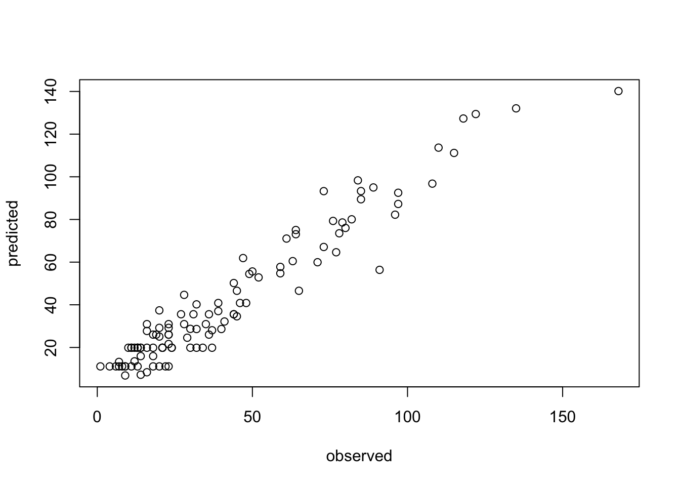
5.4.0.6 Hyperparameter tuning of random forest
| Hyperparameter | Explanation |
|---|---|
| mtry | Subset of features randomly selected in each node (from which the algorithm can select the feature that will be used to split the data). |
| minimum node size | Minimal number of observations allowed in a node (before the branching is canceled) |
| max depth | Maximum number of tree depth |
Coming back to the titanic dataset from the morning, we want to optimize the minimum node size in our RF using a simple CV.
Prepare the data:
library(EcoData)
library(dplyr)
library(missRanger)
data(titanic_ml)
data = titanic_ml
data =
  data |> select(survived, sex, age, fare, pclass)
data[,-1] = missRanger(data[,-1], verbose = 0)

data_sub =
  data |>
    mutate(age = scales::rescale(age, c(0, 1)),
           fare = scales::rescale(fare, c(0, 1))) |>
    mutate(sex = as.integer(sex) - 1L,
           pclass = as.integer(pclass - 1L))
data_new = data_sub[is.na(data_sub$survived),] # for which we want to make predictions at the end
data_obs = data_sub[!is.na(data_sub$survived),] # data with known response
data_sub$survived = as.factor(data_sub$survived)
data_obs$survived = as.factor(data_obs$survived)Hints:
- adjust the ‘
type’ argument in thepredict(…)method (the default is to predict classes) - when predicting probabilities, the randomForest will return a matrix, a column for each class, we are interested in the probability of surviving (so the second column)
Bonus:
- tune min node size (and mtry)
- use more features
Interpret: after tuning, where does the best minimum node size sit — at the smallest values, the largest, or somewhere in between? Relate the location of that optimum to the bias-variance tradeoff.
Quick check — a larger minimum node size in the random forest tends to:
library(randomForest)
set.seed(42)
data_obs = data_sub[!is.na(data_sub$survived),]
data_obs$survived = as.factor(data_obs$survived)

cv = 3
hyper_minnodesize = sample(100, 20)
split = sample.int(cv, nrow(data_obs), replace = T)

tuning_results =
    sapply(1:length(hyper_minnodesize), function(k) {
        auc_inner = NULL
        for(j in 1:cv) {
          inner_split = split == j
          train_inner = data_obs[!inner_split, ]
          test_inner = data_obs[inner_split, ]
          model = randomForest(survived~.,data = train_inner, nodesize = hyper_minnodesize[k])
          predictions = predict(model, test_inner, type = "prob")[,2]

          auc_inner[j]= Metrics::auc(test_inner$survived, predictions)
        }
      return(mean(auc_inner))
    })

results = data.frame(minnodesize = hyper_minnodesize, AUC = tuning_results)

print(results)
minnodesize AUC
1 49 0.8214663
2 65 0.8147615
3 25 0.8271051
4 74 0.8151506
5 18 0.8284641
6 100 0.8070825
7 47 0.8154820
8 24 0.8293650
9 71 0.8133736
10 89 0.8136157
11 37 0.8239713
12 20 0.8253214
13 26 0.8233802
14 3 0.8281495
15 41 0.8228877
16 27 0.8257259
17 36 0.8242946
18 5 0.8271348
19 34 0.8259364
20 87 0.8129282Make predictions:
model = randomForest(survived~.,data = data_obs, nodesize = results[which.max(results$AUC),1])

write.csv(data.frame(y = predict(model, data_new, type = "prob")[,2]), file = "Max_titanic_rf.csv")