library(keras3)

rotate = function(x){ t(apply(x, 2, rev)) }

imgPlot = function(img, title = ""){
  col = grey.colors(255)
  image(rotate(img), col = col, xlab = "", ylab = "", axes = FALSE,
     main = paste0("Label: ", as.character(title)))
}10 Convolutional Neural Networks (CNN)
The main purpose of convolutional neural networks is image recognition. (Sound can be understood as an image as well!) In a convolutional neural network, we have at least one convolution layer, additional to the normal, fully connected deep neural network layers.
Neurons in a convolution layer are connected only to a small spatially contiguous area of the input layer (receptive field). We use this structure (feature map) to scan the entire features / neurons (e.g. picture). Think of the feature map as a kernel or filter (or imagine a sliding window with weighted pixels) that is used to scan the image. As the name is already indicating, this operation is a convolution in mathematics. The kernel weights are optimized, but we use the same weights across the entire input neurons (shared weights).
The resulting (hidden) convolutional layer after training is called a feature map. You can think of the feature map as a map that shows you where the “shapes” expressed by the kernel appear in the input. One kernel / feature map will not be enough, we typically have many shapes that we want to recognize. Thus, the input layer is typically connected to several feature maps, which can be aggregated and followed by a second layer of feature maps, and so on.
You get one convolution map/layer for each kernel of one convolutional layer.
10.1 Example MNIST
We will show the use of convolutional neural networks with the MNIST data set. This data set is maybe one of the most famous image data sets. It consists of 60,000 handwritten digits from 0-9.
To do so, we define a few helper functions:
The MNIST data set is so famous that there is an automatic download function in Keras:
data = dataset_mnist()
train = data$train
test = data$test
Let’s visualize a few digits:
oldpar = par(mfrow = c(1, 3))
.n = sapply(1:3, function(x) imgPlot(train$x[x,,], train$y[x]))
par(oldpar)Similar to the normal machine learning workflow, we have to scale the pixels (from 0-255) to the range of \([0, 1]\) and one hot encode the response. For scaling the pixels, we will use arrays instead of matrices. Arrays are called tensors in mathematics and a 2D array/tensor is typically called a matrix.
train_x = array(train$x/255, c(dim(train$x), 1))
test_x = array(test$x/255, c(dim(test$x), 1))
train_y = keras3::to_categorical(train$y)
test_y = keras3::to_categorical(test$y)
The last dimension denotes the number of channels in the image. In our case we have only one channel because the images are black and white.
Most times, we would have at least 3 color channels, for example RGB (red, green, blue) or HSV (hue, saturation, value), sometimes with several additional dimensions like transparency.
To build our convolutional model, we have to specify a kernel. In our case, we will use 16 convolutional kernels (filters) of size \(2\times2\). These are 2D kernels because our images are 2D. For movies for example, one would use 3D kernels (the third dimension would correspond to time and not to the color channels).
model = keras_model_sequential(shape(28L, 28L, 1L))
model |>
 layer_conv_2d(filters = 16L,
               kernel_size = c(2L, 2L), activation = "relu") |>
 layer_max_pooling_2d() |>
 layer_conv_2d(filters = 16L, kernel_size = c(3L, 3L), activation = "relu") |>
 layer_max_pooling_2d() |>
 layer_flatten() |>
 layer_dense(100L, activation = "relu") |>
 layer_dense(10L, activation = "softmax")
summary(model)
Model: "sequential"
┏━━━━━━━━━━━━━━━━━━━━━━━━━━━━━━━━━━━┳━━━━━━━━━━━━━━━━━━━━━━━━━━┳━━━━━━━━━━━━━━━┓
┃ Layer (type) ┃ Output Shape ┃ Param # ┃
┡━━━━━━━━━━━━━━━━━━━━━━━━━━━━━━━━━━━╇━━━━━━━━━━━━━━━━━━━━━━━━━━╇━━━━━━━━━━━━━━━┩
│ conv2d (Conv2D) │ (None, 27, 27, 16) │ 80 │
├───────────────────────────────────┼──────────────────────────┼───────────────┤
│ max_pooling2d (MaxPooling2D) │ (None, 13, 13, 16) │ 0 │
├───────────────────────────────────┼──────────────────────────┼───────────────┤
│ conv2d_1 (Conv2D) │ (None, 11, 11, 16) │ 2,320 │
├───────────────────────────────────┼──────────────────────────┼───────────────┤
│ max_pooling2d_1 (MaxPooling2D) │ (None, 5, 5, 16) │ 0 │
├───────────────────────────────────┼──────────────────────────┼───────────────┤
│ flatten (Flatten) │ (None, 400) │ 0 │
├───────────────────────────────────┼──────────────────────────┼───────────────┤
│ dense (Dense) │ (None, 100) │ 40,100 │
├───────────────────────────────────┼──────────────────────────┼───────────────┤
│ dense_1 (Dense) │ (None, 10) │ 1,010 │
└───────────────────────────────────┴──────────────────────────┴───────────────┘
Total params: 43,510 (169.96 KB)
Trainable params: 43,510 (169.96 KB)
Non-trainable params: 0 (0.00 B)plot(model)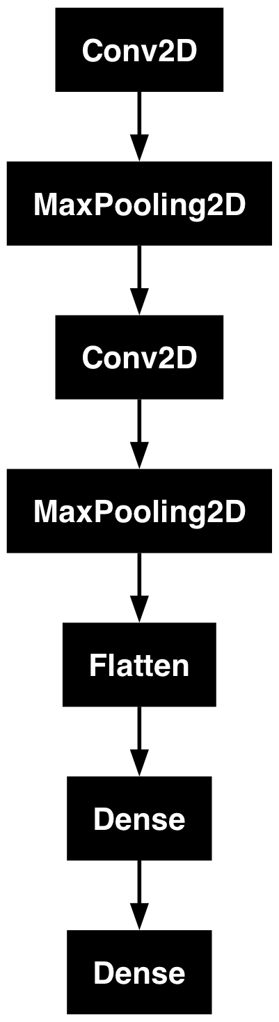
We are currently working on providing a userfriendly interface to CNN in cito:
Configure architecture:
library(cito)
architecture = create_architecture(
  conv(n_kernels = 16L, kernel_size = 2L, activation = "relu"),
  maxPool(),
  conv(n_kernels = 16L, kernel_size = 3L, activation = "relu"),
  maxPool(),
  linear(100L, activation = "relu")
  )
Prepare/download data:
library(torch)
Attaching package: 'torch'The following object is masked from 'package:keras3':
as_iteratorlibrary(torchvision)
torch_manual_seed(321L)
set.seed(123)
train_ds = mnist_dataset(
".",
download = TRUE,
train = TRUE,
transform = transform_to_tensor
)Split "train" of dataset <mnist> (~12 MB) will be downloaded and processed if
not already available.<mnist> dataset loaded with 60000 images across 10 classes.test_ds = mnist_dataset(
".",
download = TRUE,
train = FALSE,
transform = transform_to_tensor
)Split "test" of dataset <mnist> (~12 MB) will be downloaded and processed if
not already available.
<mnist> dataset loaded with 10000 images across 10 classes.Build dataloader:
train_dl = dataloader(train_ds, batch_size = 32, shuffle = TRUE)
test_dl = dataloader(test_ds, batch_size = 32)
first_batch = train_dl$.iter()
df = first_batch$.next()

df$x$size()
[1] 32 1 28 28Build convolutional neural network: We have here to calculate the shapes of our layers on our own:
We start with our input of shape (batch_size, 1, 28, 28)
sample = df$x
sample$size()
[1] 32 1 28 28First convolutional layer has shape (input channel = 1, number of feature maps = 16, kernel size = 2)
conv1 = nn_conv2d(1, 16L, 2L, stride = 1L)
(sample |> conv1())$size()
[1] 32 16 27 27Output: batch_size = 32, number of feature maps = 16, dimensions of each feature map = \((27 , 27)\) Wit a kernel size of two and stride = 1 we will lose one pixel in each dimension… Questions:
- What happens if we increase the stride?
- What happens if we increase the kernel size?
Pooling layer summarizes each feature map
(sample |> conv1() |> nnf_max_pool2d(kernel_size = 2L, stride = 2L))$size()[1] 32 16 13 13kernel_size = 2L and stride = 2L halfs the pixel dimensions of our image.
Fully connected layer
Now we have to flatten our final output of the convolutional neural network model to use a normal fully connected layer, but to do so we have to calculate the number of inputs for the fully connected layer:
dims = (sample |> conv1() |>
          nnf_max_pool2d(kernel_size = 2L, stride = 2L))$size()
# Without the batch size of course.
final = prod(dims[-1])
print(final)
[1] 2704fc = nn_linear(final, 10L)
(sample |> conv1() |> nnf_max_pool2d(kernel_size = 2L, stride = 2L)
|> torch_flatten(start_dim = 2L) |> fc())$size()[1] 32 10Build the network:
net = nn_module(
  "mnist",
  initialize = function(){
    self$conv1 = nn_conv2d(1, 16L, 2L)
    self$conv2 = nn_conv2d(16L, 16L, 3L)
    self$fc1 = nn_linear(400L, 100L)
    self$fc2 = nn_linear(100L, 10L)
  },
  forward = function(x){
    x |>
      self$conv1() |> # output dim: 16, 27, 27
      nnf_relu() |>
      nnf_max_pool2d(2) |> # output dim: 16, 13, 13
      self$conv2() |> # output dim: 16, 11, 11
      nnf_relu() |>
      nnf_max_pool2d(2) |> # output dim: 16, 5, 5
      torch_flatten(start_dim = 2) |> # 16*5*5
      self$fc1() |>
      nnf_relu() |>
      self$fc2()
  }
)
We additionally used a pooling layer for downsizing the resulting feature maps. Without further specification, a \(2\times2\) pooling layer is taken automatically. Pooling layers take the input feature map and divide it into (in our case) parts of \(2\times2\) size. Then the respective pooling operation is executed. For every input map/layer, you get one (downsized) output map/layer.
As we are using the max pooling layer (there are sever other methods like the mean pooling), only the maximum value of these 4 parts is taken and forwarded further. Example input:
1   2   |   5   8   |   3   6
6   5   |   2   4   |   8   1
------------------------------
9   4   |   3   7   |   2   5
0   3   |   2   7   |   4   9
We use max pooling for every field:
max(1, 2, 6, 5)   |   max(5, 8, 2, 4)   |   max(3, 6, 8, 1)
-----------------------------------------------------------
max(9, 4, 0, 3)   |   max(3, 7, 2, 7)   |   max(2, 5, 4, 9)
So the resulting pooled information is:
6   |   8   |   8
------------------
9   |   7   |   9
In this example, a \(4\times6\) layer was transformed to a \(2\times3\) layer and thus downsized. This is similar to the biological process called lateral inhibition where active neurons inhibit the activity of neighboring neurons. It’s a loss of information but often very useful for aggregating information and prevent overfitting.
After another convolution and pooling layer, we flatten the output. This means that the following dense layer treats the previous layer as a full layer (so the dense layer is connected to all the weights from the last feature maps). You can think of this as transforming a matrix (2D) into a simple 1D vector. The full vector is then used. After flattening the layer, we can simply use our typical output layer.
The rest is as usual:
First we compile the model:
model |>
  keras3::compile(
      optimizer = keras3::optimizer_adamax(0.01),
      loss = keras3::loss_categorical_crossentropy
  )
summary(model)
Model: "sequential"
┏━━━━━━━━━━━━━━━━━━━━━━━━━━━━━━━━━━━┳━━━━━━━━━━━━━━━━━━━━━━━━━━┳━━━━━━━━━━━━━━━┓
┃ Layer (type) ┃ Output Shape ┃ Param # ┃
┡━━━━━━━━━━━━━━━━━━━━━━━━━━━━━━━━━━━╇━━━━━━━━━━━━━━━━━━━━━━━━━━╇━━━━━━━━━━━━━━━┩
│ conv2d (Conv2D) │ (None, 27, 27, 16) │ 80 │
├───────────────────────────────────┼──────────────────────────┼───────────────┤
│ max_pooling2d (MaxPooling2D) │ (None, 13, 13, 16) │ 0 │
├───────────────────────────────────┼──────────────────────────┼───────────────┤
│ conv2d_1 (Conv2D) │ (None, 11, 11, 16) │ 2,320 │
├───────────────────────────────────┼──────────────────────────┼───────────────┤
│ max_pooling2d_1 (MaxPooling2D) │ (None, 5, 5, 16) │ 0 │
├───────────────────────────────────┼──────────────────────────┼───────────────┤
│ flatten (Flatten) │ (None, 400) │ 0 │
├───────────────────────────────────┼──────────────────────────┼───────────────┤
│ dense (Dense) │ (None, 100) │ 40,100 │
├───────────────────────────────────┼──────────────────────────┼───────────────┤
│ dense_1 (Dense) │ (None, 10) │ 1,010 │
└───────────────────────────────────┴──────────────────────────┴───────────────┘
Total params: 43,510 (169.96 KB)
Trainable params: 43,510 (169.96 KB)
Non-trainable params: 0 (0.00 B)Then, we train the model:
library(tensorflow)
library(keras3)

epochs = 5L
batch_size = 32L
model |>
  fit(
    x = train_x,
    y = train_y,
    epochs = epochs,
    batch_size = batch_size,
    shuffle = TRUE,
    validation_split = 0.2
  )
Fit model:
# Note: cito wants the channels on the second position!
model.cito = cnn(X = aperm(train_x, c(1, 4, 2, 3)),
                 Y = as.factor(apply(train_y, 1, which.max)),
                 loss = "softmax",
                 architecture = architecture,
                 batchsize = 128L,
                 epochs = 5L,
                 optimizer = "adam")
Warning in get_loss(loss, Y, custom_parameters, baseloss): loss = 'softmax' is
deprecated and will be removed in a future version of 'cito'. Please use loss =
'cross-entropy' instead.Loss at epoch 1: 0.268981, lr: 0.01000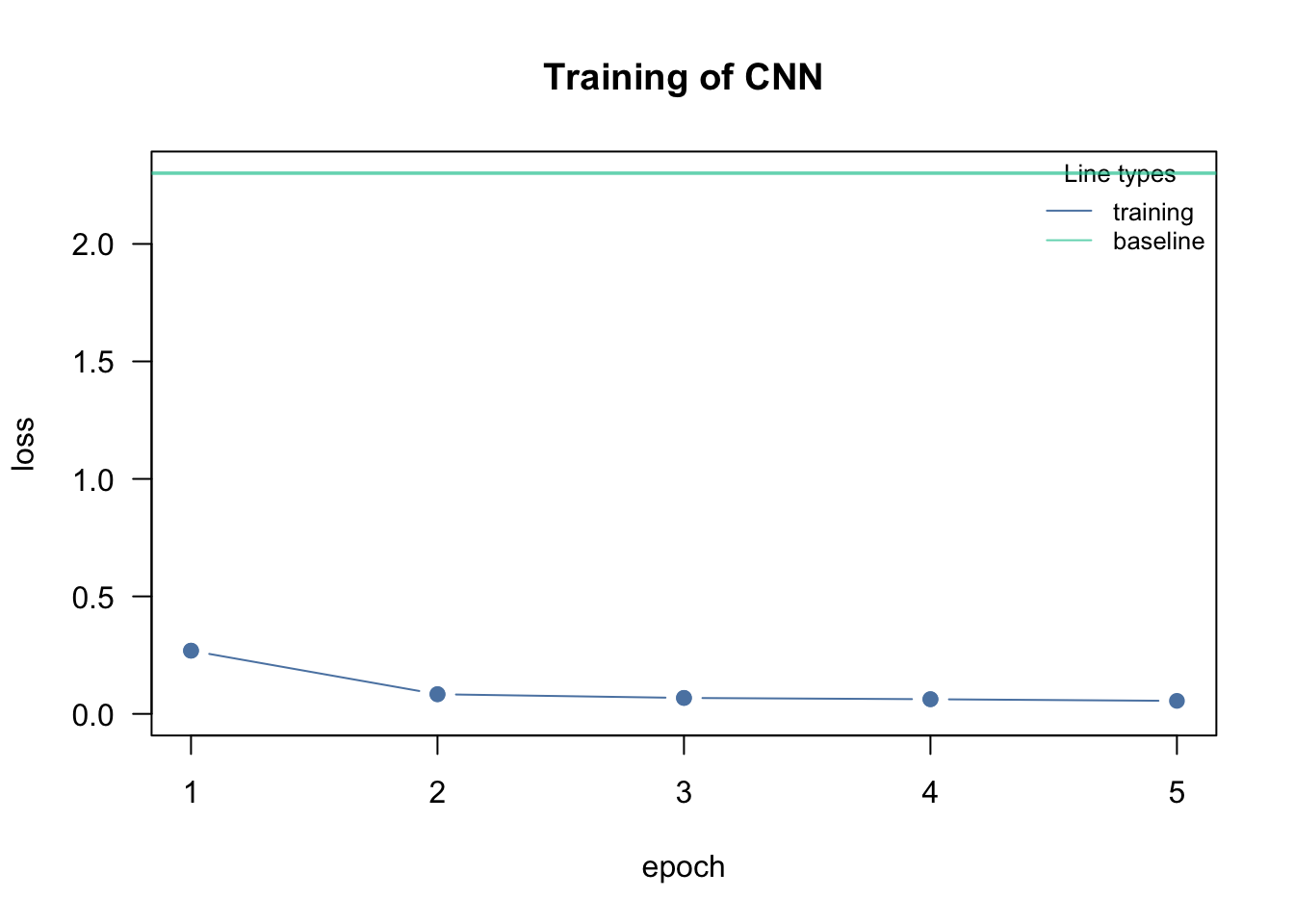
Loss at epoch 2: 0.083697, lr: 0.01000
Loss at epoch 3: 0.067905, lr: 0.01000
Loss at epoch 4: 0.062421, lr: 0.01000
Loss at epoch 5: 0.055394, lr: 0.01000
Visualize model:
plot(model.cito)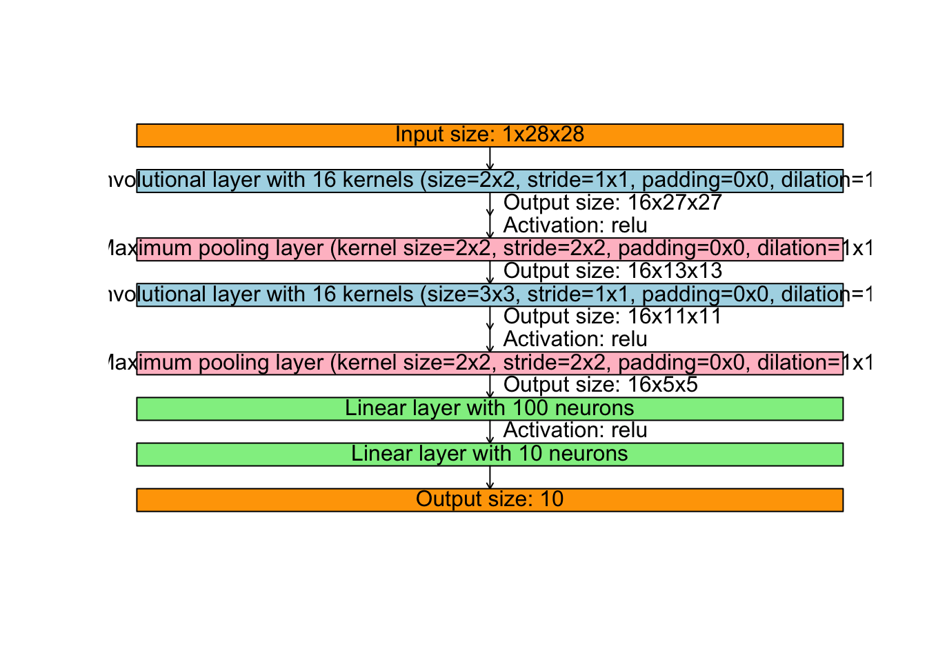
Evaluation:
pred = predict(model.cito, newdata = aperm(test_x, c(1, 4, 2, 3)), type = "response")
mean(apply(test_y, 1, which.max) == apply(pred, 1, which.max))
[1] 0.9813Train model:
library(torch)
torch_manual_seed(321L)
set.seed(123)

model_torch = net()
opt = optim_adam(params = model_torch$parameters, lr = 0.01)

for(e in 1:3){
  losses = c()
  coro::loop(
    for(batch in train_dl){
      opt$zero_grad()
      pred = model_torch(batch[[1]])
      loss = nnf_cross_entropy(pred, batch[[2]], reduction = "mean")
      loss$backward()
      opt$step()
      losses = c(losses, loss$item())
    }
  )
  cat(sprintf("Loss at epoch %d: %3f\n", e, mean(losses)))
}
Evaluation:
model_torch$eval()

test_losses = c()
total = 0
correct = 0

coro::loop(
  for(batch in test_dl){
    output = model_torch(batch[[1]])
    labels = batch[[2]]
    loss = nnf_cross_entropy(output, labels)
    test_losses = c(test_losses, loss$item())
    predicted = torch_max(output$data(), dim = 2)[[2]]
    total = total + labels$size(1)
    correct = correct + (predicted == labels)$sum()$item()
  }
)

mean(test_losses)
test_accuracy =  correct/total
test_accuracy
10.2 Example CIFAR
CIFAR10 is another famous image classification dataset. It consists of ten classes with colored images (see https://www.cs.toronto.edu/~kriz/cifar.html).
Prepare data, now with 3 channels (colored images):
library(keras3)
data = keras3::dataset_cifar10()
train = data$train
test = data$test
image = train$x[1,,,]
image |>
 image_to_array() |>
  (\(x) x / 255)() |>
 as.raster() |>
 plot()
## normalize pixel to 0-1
train_x = array(train$x/255, c(dim(train$x)))
test_x = array(test$x/255, c(dim(test$x)))
train_y = keras3::to_categorical(train$y)
test_y = keras3::to_categorical(test$y)
model = keras_model_sequential(shape(32L, 32L,3L))
model |>
 layer_conv_2d(input_shape = c(32L, 32L,3L),filters = 16L, kernel_size = c(2L,2L), activation = "relu") |>
 layer_max_pooling_2d() |>
 layer_dropout(0.3) |>
 layer_conv_2d(filters = 16L, kernel_size = c(3L,3L), activation = "relu") |>
 layer_max_pooling_2d() |>
 layer_flatten() |>
 layer_dense(10, activation = "softmax")
summary(model)
model |>
 compile(
 optimizer = optimizer_adamax(),
 loss = keras3::loss_categorical_crossentropy
 )
early = callback_early_stopping(patience = 5L)
epochs = 1L
batch_size =20L
model |> fit(
 x = train_x,
 y = train_y,
 epochs = epochs,
 batch_size = batch_size,
 shuffle = TRUE,
 validation_split = 0.2,
 callbacks = c(early)
)
train_ds = cifar10_dataset(
".",
download = TRUE,
train = TRUE,
transform = transform_to_tensor
)Split "train" of dataset <cifar10_dataset> (~160 MB) will be downloaded and
processed if not already available.
<cifar10_dataset> dataset loaded with 50000 images across 11 classes.test_ds = cifar10_dataset(
".",
download = TRUE,
train = FALSE,
transform = transform_to_tensor
)Split "test" of dataset <cifar10_dataset> (~160 MB) will be downloaded and
processed if not already available.
<cifar10_dataset> dataset loaded with 10000 images across 11 classes.train_dl = dataloader(train_ds, batch_size = 32, shuffle = TRUE)
test_dl = dataloader(test_ds, batch_size = 32)
first_batch = train_dl$.iter()
df = first_batch$.next()
df$x$size()[1] 32 3 32 32Model:
net = nn_module(
  "mnist",
  initialize = function(dropout_rate = 0.3){
    self$conv1 = nn_conv2d(3, 8L, 2L) # 8, 31, 31 -> 8, 15, 15
    self$dropout1 = nn_dropout2d(p = dropout_rate)
    self$conv2 = nn_conv2d(8L, 16L, 3L) # 16, 13, 13 -> 16, 6, 6
    self$dropout2 = nn_dropout2d(p = dropout_rate)
    self$conv3 = nn_conv2d(16L, 32L, 3L) # 32, 4, 4 -> 32, 2, 2
    self$dropout3 = nn_dropout2d(p = dropout_rate)
    self$fc1 = nn_linear(128L, 10L)
  },
  forward = function(x){
    x |>
      self$conv1() |>
      nnf_relu() |>
      self$dropout1() |>
      nnf_max_pool2d(2) |>
      self$conv2() |>
      nnf_relu() |>
      self$dropout2() |>
      nnf_max_pool2d(2) |>
      self$conv3() |>
      self$dropout3() |>
      nnf_max_pool2d(2) |>
      torch_flatten(start_dim = 2) |>
      self$fc1()
  }
)
Train model:
model_torch = net()
opt = optim_adam(params = model_torch$parameters, lr = 0.01)

for(e in 1:3){
  losses = c()
  coro::loop(
    for(batch in train_dl){
      opt$zero_grad()
      pred = model_torch(batch[[1]])
      loss = nnf_cross_entropy(pred, batch[[2]], reduction = "mean")
      loss$backward()
      opt$step()
      losses = c(losses, loss$item())
    }
  )
  cat(sprintf("Loss at epoch %d: %3f\n", e, mean(losses)))
}
train_x = array(train$x/255, c(dim(train$x)))
test_x = array(test$x/255, c(dim(test$x)))
train_y = keras3::to_categorical(train$y)
test_y = keras3::to_categorical(test$y)
train_x = aperm(train_x, c(1, 4, 2, 3))
test_x = aperm(test_x, c(1, 4, 2, 3))
architecture = create_architecture(
conv(n_kernels = 32, kernel_size = 2L, activation = "relu"),
maxPool(),
conv(n_kernels = 16, kernel_size = 3L, activation = "relu"),
maxPool(),
default_dropout = 0.2
)
model.cito = cnn(X = train_x,
Y = as.factor(apply(train_y, 1, which.max)),
loss = "softmax",
architecture = architecture,
batchsize = 128L,
epochs = 5L,
validation = 0.2,
optimizer = "adam",
lr = 0.001)Warning in get_loss(loss, Y, custom_parameters, baseloss): loss = 'softmax' is
deprecated and will be removed in a future version of 'cito'. Please use loss =
'cross-entropy' instead.Loss at epoch 1: training: 1.957, validation: 1.704, lr: 0.00100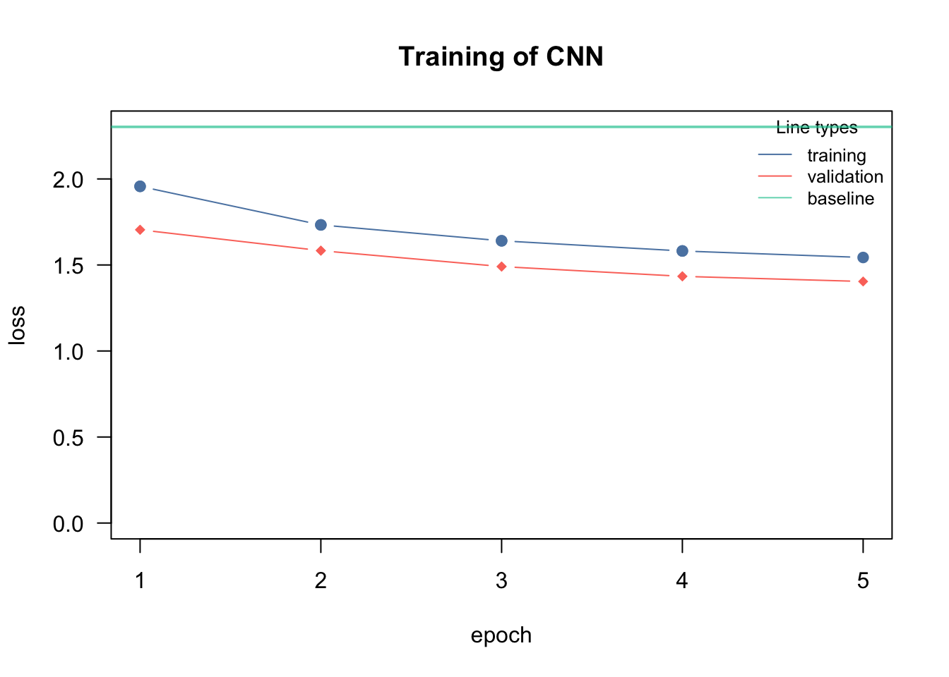
Loss at epoch 2: training: 1.733, validation: 1.583, lr: 0.00100
Loss at epoch 3: training: 1.640, validation: 1.491, lr: 0.00100
Loss at epoch 4: training: 1.581, validation: 1.434, lr: 0.00100
Loss at epoch 5: training: 1.544, validation: 1.404, lr: 0.00100
Architecture:
plot(model.cito)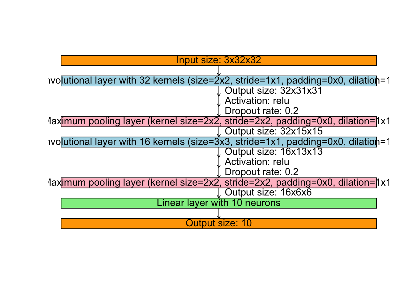
Explainable AI:
library(torch)
observation = 19
Xt = torch::torch_tensor(train_x[1:20,,,], requires_grad = TRUE)
pred = model.cito$net(Xt)
grads = torch::autograd_grad(pred[,apply(train_y, 1, which.max)[observation],drop=F], Xt, grad_outputs = torch_ones(20, 32))

old_par = par()
par(mfrow = c(2, 2))
for(i in 1:3) fields::image.plot(as.array(grads[[1]]) [observation,i,,])
image = aperm(train_x[observation,,,]*255., c(2, 3, 1))
image |>
 image_to_array() |>
  (\(x) x / 255)() |>
 as.raster() |>
 plot()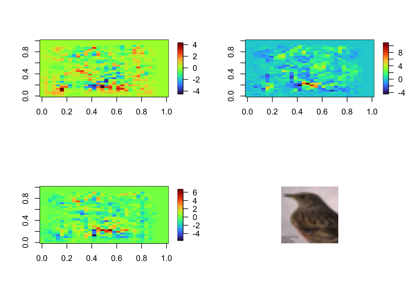
par(old_par)Warning in par(old_par): graphical parameter "cin" cannot be setWarning in par(old_par): graphical parameter "cra" cannot be setWarning in par(old_par): graphical parameter "csi" cannot be setWarning in par(old_par): graphical parameter "cxy" cannot be setWarning in par(old_par): graphical parameter "din" cannot be setWarning in par(old_par): graphical parameter "page" cannot be set10.3 Exercise
10.3.0.1 Task: CNN for flower dataset
The next exercise is based on the flower dataset in the Ecodata package.
Follow the steps above and build your own convolutional neural network.
Finally, submit your predictions to the submission server. If you have extra time, take a look at kaggle and find the flower dataset challenge for specific architectures tailored for this dataset.
Tasks:
- If you are unsure how do it, take a look at the solution and try to make the model more complex (e.g. add convolutional layers, regularization, etc.)
- Take a look at this notebook from kaggle , try to copy their architecture (it is the same dataset but upsized (i.e. more pixels, the only difference is the input dimension))
Prepare data:
library(tensorflow)
library(keras3)

# keras
train = EcoData::dataset_flower()$train/255
test = EcoData::dataset_flower()$test/255
labels = EcoData::dataset_flower()$labels

# torch / cito -> channels must be at the second dim
train_torch = aperm(train, c(1, 4, 2, 3))
test_torch = aperm(test, c(1, 4, 2, 3))
Plot flower:
train[100,,,] |>
  image_to_array() |>
  as.raster() |>
  plot()
Tip: Take a look at the dataset chapter.
Build model:
net = nn_module(
  "flower",
  initialize = function(dropout_rate = 0.3){
    self$conv1 = nn_conv2d(3, 8L, 4L) # 8, 77, 77 -> 8, 19, 19
    self$dropout1 = nn_dropout2d(p = dropout_rate)
    self$fc1 = nn_linear(2888, 5L)
  },
  forward = function(x){
    x |>
      self$conv1() |>
      nnf_relu() |>
      self$dropout1() |>
      nnf_max_pool2d(4) |>
      torch_flatten(start_dim = 2) |>
      self$fc1()
  }
)

model_torch = net()
opt = optim_adam(params = model_torch$parameters, lr = 0.01)

dataset = tensor_dataset(torch_tensor(train_torch),
                         torch_tensor(labels+1, dtype = torch_long())
                         )
train_dl = torch::dataloader(dataset, batch_size = 50L, shuffle = TRUE)

for(e in 1:3){
  losses = c()
  coro::loop(
    for(batch in train_dl){
      opt$zero_grad()
      pred = model_torch(batch[[1]])
      loss = nnf_cross_entropy(pred, batch[[2]], reduction = "mean")
      loss$backward()
      opt$step()
      losses = c(losses, loss$item())
    }
  )
  cat(sprintf("Loss at epoch %d: %3f\n", e, mean(losses)))
}
Loss at epoch 1: 1.617379
Loss at epoch 2: 1.441577
Loss at epoch 3: 1.454987Predictions:
# Prediction on training data:
model_torch$eval()
predictions = model_torch(torch_tensor(train_torch))
predictions = nnf_softmax( predictions, 2) |> as_array() # apply link function
pred = apply(predictions, 1, which.max)
Metrics::accuracy(pred - 1L, labels)
[1] 0.4634469table(pred)pred
1 2 3 4 5
121 1377 374 775 376 # Prediction for the submission server:
predictions = model_torch(torch_tensor(test_torch))
predictions = nnf_softmax( predictions, 2) |> as_array() # apply link function
pred = predictions |> apply(1, which.max) - 1L
table(pred)pred
0 1 2 3 4
59 581 175 323 162 write.csv(data.frame(y = pred), file = "cnn.csv")Build model:
model = keras_model_sequential(shape(80L, 80L, 3L))
model |>
  layer_conv_2d(filters = 4L, kernel_size = 2L) |>
  layer_max_pooling_2d() |>
  layer_flatten() |>
  layer_dense(units = 5L, activation = "softmax")

### Model fitting ###

model |>
  compile(loss = loss_categorical_crossentropy,
          optimizer = optimizer_adamax(learning_rate = 0.01))

model |>
  fit(x = train, y = keras3::to_categorical(labels, 5L))
95/95 - 0s - 3ms/step - loss: 2.1091Predictions:
# Prediction on training data:
pred = apply(model |> predict(train), 1, which.max)
95/95 - 0s - 901us/stepMetrics::accuracy(pred - 1L, labels)[1] 0.5362223table(pred)pred
1 2 3 4 5
841 580 656 248 698 # Prediction for the submission server:
pred = model |> predict(test) |> apply(1, which.max) - 1L41/41 - 0s - 801us/steptable(pred)pred
0 1 2 3 4
346 236 290 100 328 architecture = create_architecture(
conv(n_kernels = 8L, kernel_size = 2L, activation = "relu"),
maxPool(),
default_dropout = 0.2
)
model.cito = cnn(X = aperm(train, c(1, 4, 2, 3)) ,
Y = as.factor(labels+1L),
loss = "softmax",
architecture = architecture,
batchsize = 128L,
epochs = 5L,
validation = 0.2,
optimizer = "adam",
lr = 0.001)Warning in get_loss(loss, Y, custom_parameters, baseloss): loss = 'softmax' is
deprecated and will be removed in a future version of 'cito'. Please use loss =
'cross-entropy' instead.Loss at epoch 1: training: 1.556, validation: 1.351, lr: 0.00100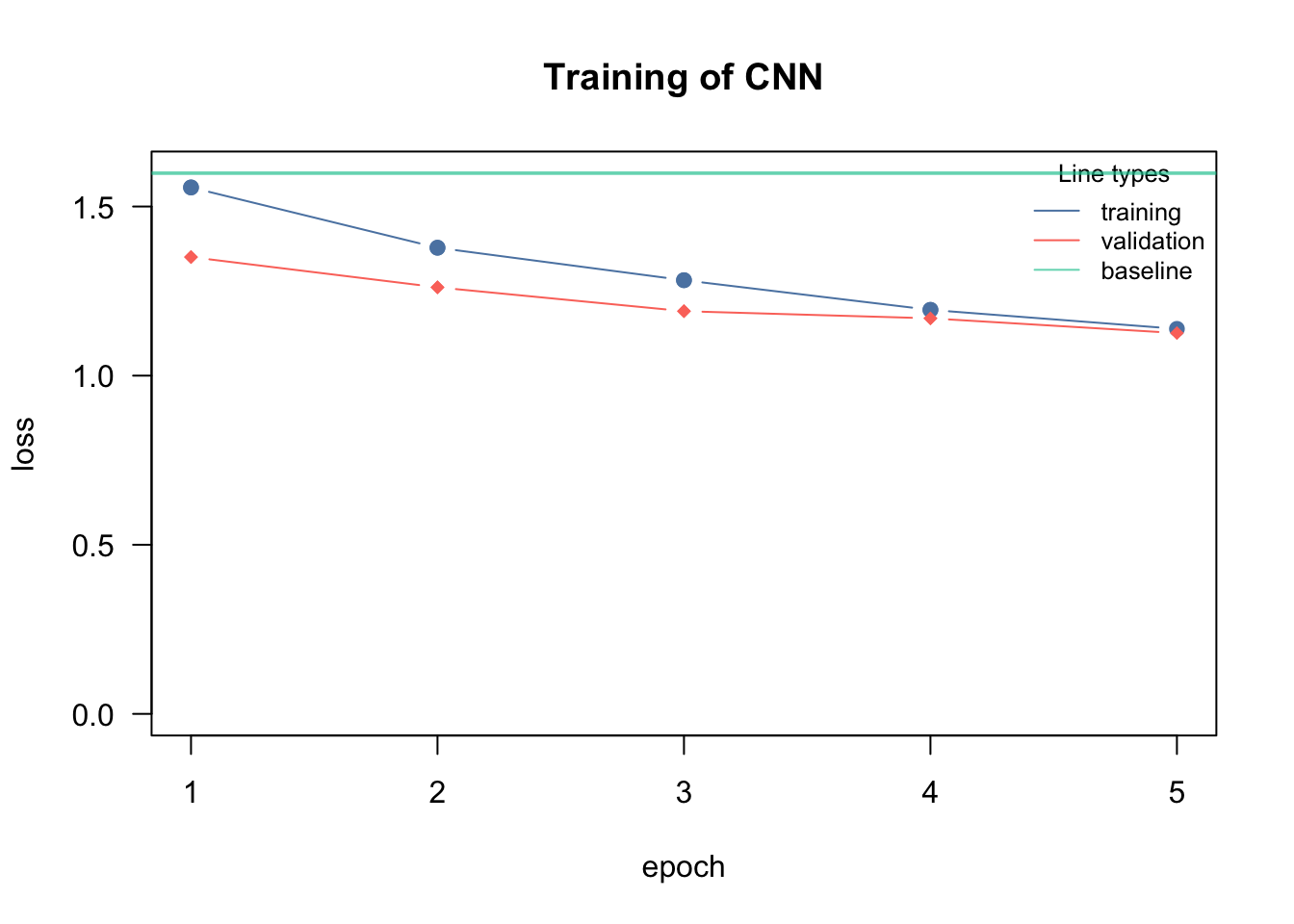
Loss at epoch 2: training: 1.378, validation: 1.261, lr: 0.00100
Loss at epoch 3: training: 1.282, validation: 1.191, lr: 0.00100
Loss at epoch 4: training: 1.195, validation: 1.169, lr: 0.00100
Loss at epoch 5: training: 1.138, validation: 1.126, lr: 0.00100
pred = predict(model.cito, newdata = aperm(test, c(1, 4, 2, 3)), type = "response") |> apply(1, which.max) - 1LSubmission:
write.csv(data.frame(y = pred), file = "cnn.csv")10.3.0.2 Task: CNN for the SDM dataset
The next exercise is based on the SDM dataset
Follow the steps above and build your own convolutional neural network.
Finally, submit your predictions to the submission server. If you have extra time, take a look at kaggle and find the SDM dataset challenge for specific architectures tailored for this dataset.
Hint: Take a look at the loss_binary_focal_crossentropy function from the keras package!
Prepare data:
load("sdm.RData")

# keras
train = sdm_img$train/max(sdm_img$train, sdm_img$test, na.rm = TRUE)
test = sdm_img$test/max(sdm_img$test, sdm_img$test, na.rm = TRUE)
train[is.na(train)] = 0
test[is.na(test)] = 0
train = aperm(train, c(1, 3, 4, 2))
test = aperm(test, c(1, 3, 4, 2))

labels = Y_train

# torch / cito -> channels must be at the second dim
train_torch = aperm(train, c(1, 4, 2, 3))
test_torch = aperm(test, c(1, 4, 2, 3))
Plot flower:
train[102,,,] |>
  image_to_array() |>
  as.raster() |>
  plot()
Tip: Take a look at the dataset chapter.
Build model:
net = nn_module(
  "sdm",
  initialize = function(dropout_rate = 0.3){
    self$conv1 = nn_conv2d(4, 8L, 4L) # 8, 77, 77 -> 8, 19, 19
    self$dropout1 = nn_dropout2d(p = dropout_rate)
    self$fc1 = nn_linear(1800, ncol(Y_train))
  },
  forward = function(x){
    x |>
      self$conv1() |>
      nnf_relu() |>
      self$dropout1() |>
      nnf_max_pool2d(4) |>
      torch_flatten(start_dim = 2) |>
      self$fc1() |>
      torch_sigmoid()
  }
)

model_torch = net()
opt = optim_adam(params = model_torch$parameters, lr = 0.01)

dataset = tensor_dataset(torch_tensor(train_torch),
                         torch_tensor(labels, dtype = torch_float())
                         )
train_dl = torch::dataloader(dataset, batch_size = 50L, shuffle = TRUE)

for(e in 1:3){
  losses = c()
  coro::loop(
    for(batch in train_dl){
      opt$zero_grad()
      pred = model_torch(batch[[1]])
      loss = nnf_binary_cross_entropy(pred, batch[[2]], reduction = "mean")
      loss$backward()
      opt$step()
      losses = c(losses, loss$item())
    }
  )
  cat(sprintf("Loss at epoch %d: %3f\n", e, mean(losses)))
}
Loss at epoch 1: 0.148927
Loss at epoch 2: 0.134455
Loss at epoch 3: 0.129533Predictions:
# Prediction on training data:
model_torch$eval()
predictions = model_torch(torch_tensor(train_torch))  |> as_array()

aucs = sapply(1:ncol(Y_train), function(i) Metrics::auc(Y_train[,i], predictions[,i]))
mean(aucs)
[1] 0.7033492predictions = model_torch(torch_tensor(test_torch)) |> as_array()
write.csv(data.frame(y = as.vector(predictions)), file = "cnn.csv")Build model:
model = keras_model_sequential(shape(64, 64, 4L))
model |>
  layer_conv_2d(filters = 4L, kernel_size = 2L) |>
  layer_max_pooling_2d() |>
  layer_flatten() |>
  layer_dense(units = ncol(Y_train), activation = "sigmoid")

### Model fitting ###

model |>
  compile(loss = loss_binary_crossentropy, # check out the loss_binary_focal_crossentropy!!!
          optimizer = optimizer_adamax(learning_rate = 0.01))

model |>
  fit(x = train, y = labels)
313/313 - 1s - 3ms/step - loss: 0.1285Predictions:
# Prediction on training data:
predictions = model |> predict(train)
313/313 - 0s - 944us/stepaucs = sapply(1:ncol(Y_train), function(i) Metrics::auc(Y_train[,i], predictions[,i]))
mean(aucs)[1] 0.664461# Prediction for the submission server:
predictions = model |> predict(test)63/63 - 0s - 1ms/stepwrite.csv(data.frame(y = as.vector(predictions)), file = "cnn.csv")architecture = create_architecture(
conv(n_kernels = 8L, kernel_size = 2L, activation = "relu"),
maxPool(),
default_dropout = 0.2
)
model.cito = cnn(X = train_torch ,
Y = labels,
loss = "bernoulli",
architecture = architecture,
batchsize = 128L,
epochs = 5L,
validation = 0.2,
optimizer = "adam",
lr = 0.001)Loss at epoch 1: training: 0.187, validation: 0.127, lr: 0.00100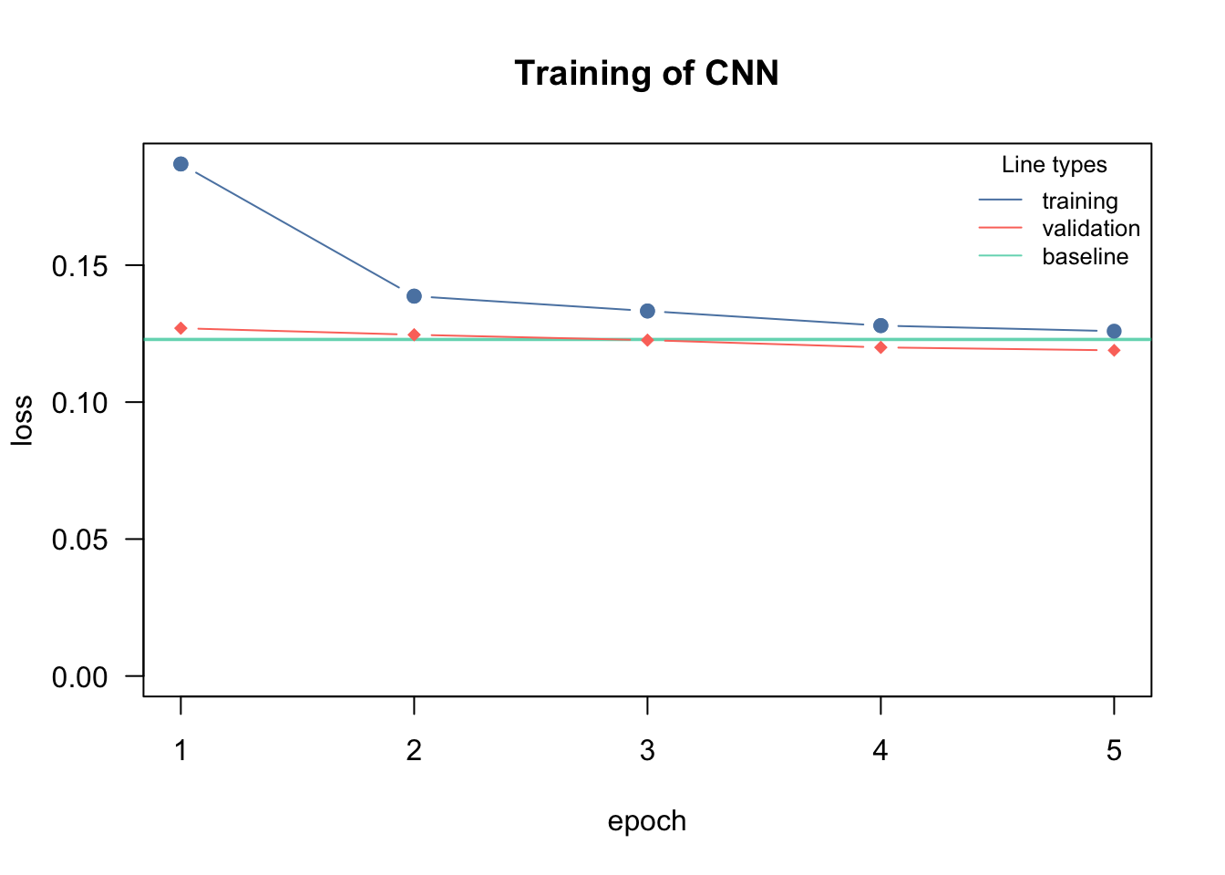
Loss at epoch 2: training: 0.139, validation: 0.125, lr: 0.00100
Loss at epoch 3: training: 0.133, validation: 0.123, lr: 0.00100
Loss at epoch 4: training: 0.128, validation: 0.120, lr: 0.00100
Loss at epoch 5: training: 0.126, validation: 0.119, lr: 0.00100predictions = model.cito |> predict(train_torch)
aucs = sapply(1:ncol(Y_train), function(i) Metrics::auc(Y_train[,i], predictions[,i]))
mean(aucs)
[1] 0.7102078Submission:
predictions = model.cito |> predict(test_torch)
write.csv(data.frame(y = as.vector(predictions)), file = "cnn.csv")
10.4 Advanced Training Techniques
10.4.1 Data Augmentation
Having to train a convolutional neural network using very little data is a common problem. Data augmentation helps to artificially increase the number of images.
The idea is that a convolutional neural network learns specific structures such as edges from images. Rotating, adding noise, and zooming in and out will preserve the overall key structure we are interested in, but the model will see new images and has to search once again for the key structures.
Luckily, it is very easy to use data augmentation in Keras.
To show this, we will use our flower data set. We have to define a generator object (a specific object which infinitely draws samples from our data set). In the generator we can turn on the data augmentation.
reticulate::use_virtualenv("r-keras")
library(keras3)
library(tensorflow)
library(tfdatasets)
Attaching package: 'tfdatasets'The following object is masked from 'package:torch':
as_iteratorThe following object is masked from 'package:keras3':
shapedata = EcoData::dataset_flower()
train = data$train/255
labels = data$labels
# data augemention model
aug = keras_model_sequential()
aug |>
layer_random_flip() |>
layer_random_rotation(factor = c(-0.5, 0.5)) |>
layer_random_brightness(factor = c(-0.5, 0.5), value_range = c(0, 1))
augModel: "sequential_3"
┏━━━━━━━━━━━━━━━━━━━━━━━━━━━━━━━━━━━┳━━━━━━━━━━━━━━━━━━━━━━━━━━┳━━━━━━━━━━━━━━━┓
┃ Layer (type) ┃ Output Shape ┃ Param # ┃
┡━━━━━━━━━━━━━━━━━━━━━━━━━━━━━━━━━━━╇━━━━━━━━━━━━━━━━━━━━━━━━━━╇━━━━━━━━━━━━━━━┩
│ random_flip (RandomFlip) │ ? │ 0 (unbuilt) │
├───────────────────────────────────┼──────────────────────────┼───────────────┤
│ random_rotation (RandomRotation) │ ? │ 0 (unbuilt) │
├───────────────────────────────────┼──────────────────────────┼───────────────┤
│ random_brightness │ ? │ 0 (unbuilt) │
│ (RandomBrightness) │ │ │
└───────────────────────────────────┴──────────────────────────┴───────────────┘
Total params: 0 (0.00 B)
Trainable params: 0 (0.00 B)
Non-trainable params: 0 (0.00 B)# Prepare datasets
dataset = tfdatasets::tensor_slices_dataset(list(train, to_categorical(labels)))
dataset <- dataset |>
dataset_map(function(x, y) list(aug(x), y))
batch_size <- 64
train_ds <- dataset |>
dataset_batch(batch_size) |>
dataset_prefetch(buffer_size = tf$data$AUTOTUNE)
# test!
batch <- train_ds |>
dataset_take(1) |>
as_iterator() |>
iter_next()
as.array(batch[[1]][1,,,]) |>
image_to_array() |>
as.raster() |>
plot()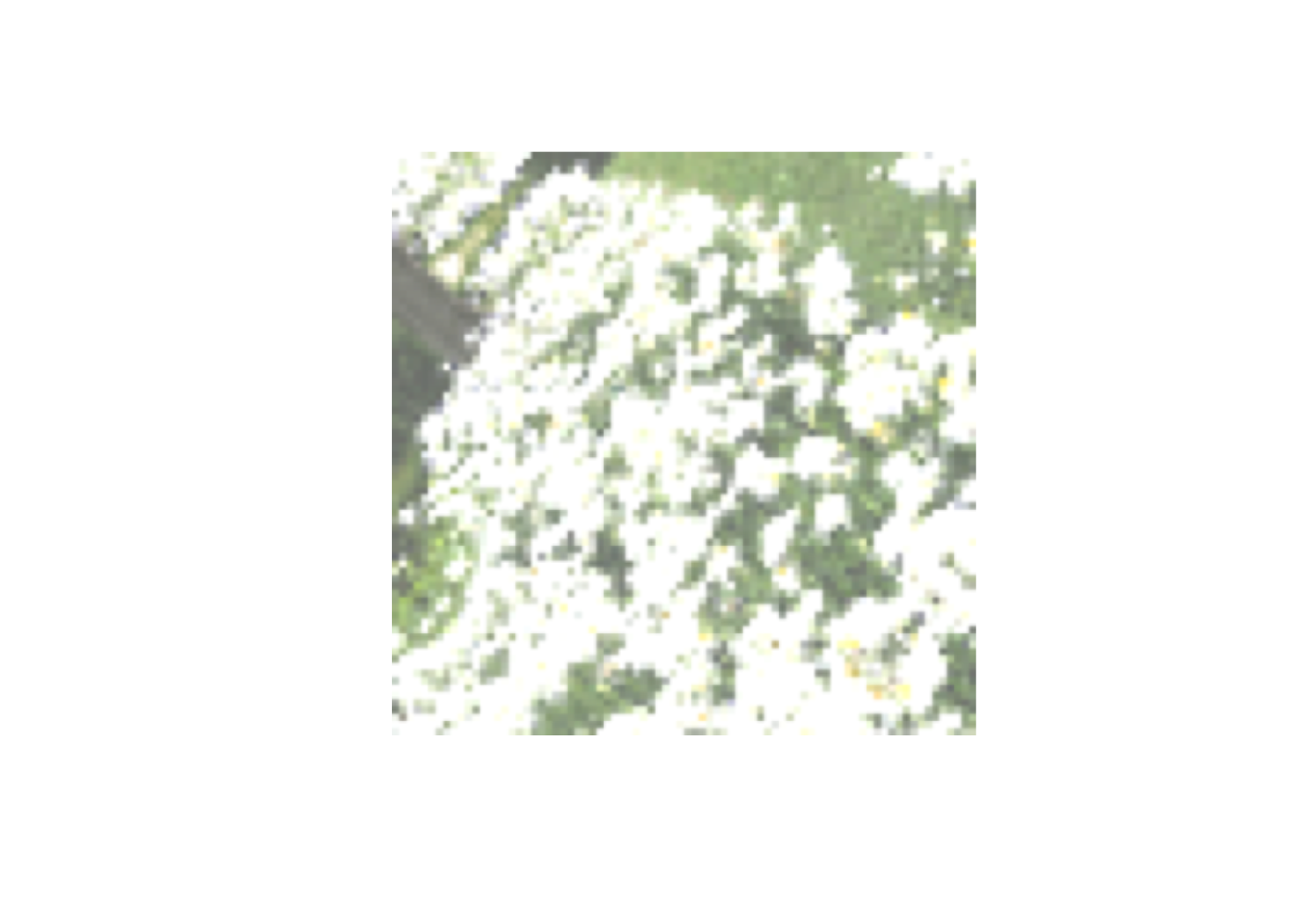
# model fitting
model = keras_model_sequential(shape(80L, 80L, 3L))
model |>
layer_conv_2d(filters = 4L, kernel_size = 2L) |>
layer_max_pooling_2d() |>
layer_flatten() |>
layer_dense(units = 5L, activation = "softmax")
model |>
keras3::compile(loss = keras3::loss_categorical_crossentropy,
optimizer = keras3::optimizer_adamax(learning_rate = 0.01))
model |> fit(train_ds, epochs = 2L)Epoch 1/2
48/48 - 1s - 18ms/step - loss: 19.6252
Epoch 2/2
48/48 - 1s - 15ms/step - loss: 26.7452Using data augmentation we can artificially increase the number of images.
In Torch, we have to change the transform function (but only for the train dataloader):
library(torch)
torch_manual_seed(321L)
set.seed(123)
net = nn_module(
"flower",
initialize = function(dropout_rate = 0.3){
self$conv1 = nn_conv2d(3, 8L, 4L) # 8, 77, 77 -> 8, 19, 19
self$dropout1 = nn_dropout2d(p = dropout_rate)
self$fc1 = nn_linear(2888, 5L)
},
forward = function(x){
x |>
self$conv1() |>
nnf_relu() |>
self$dropout1() |>
nnf_max_pool2d(4) |>
torch_flatten(start_dim = 2) |>
self$fc1()
}
)
train_transforms = function(img){
img |>
transform_to_tensor() |>
transform_random_horizontal_flip(p = 0.3) |>
transform_random_resized_crop(size = c(28L, 28L)) |>
transform_random_vertical_flip(0.3)
}
train_ds = mnist_dataset(".", download = TRUE, train = TRUE,
transform = train_transforms)
test_ds = mnist_dataset(".", download = TRUE, train = FALSE,
transform = transform_to_tensor)
train_dl = dataloader(train_ds, batch_size = 100L, shuffle = TRUE)
test_dl = dataloader(test_ds, batch_size = 100L)
model_torch = net()
opt = optim_adam(params = model_torch$parameters, lr = 0.01)
for(e in 1:1){
losses = c()
coro::loop(
for(batch in train_dl){
opt$zero_grad()
pred = model_torch(batch[[1]])
loss = nnf_cross_entropy(pred, batch[[2]], reduction = "mean")
loss$backward()
opt$step()
losses = c(losses, loss$item())
}
)
cat(sprintf("Loss at epoch %d: %3f\n", e, mean(losses)))
}
model_torch$eval()
test_losses = c()
total = 0
correct = 0
coro::loop(
for(batch in test_dl){
output = model_torch(batch[[1]])
labels = batch[[2]]
loss = nnf_cross_entropy(output, labels)
test_losses = c(test_losses, loss$item())
predicted = torch_max(output$data(), dim = 2)[[2]]
total = total + labels$size(1)
correct = correct + (predicted == labels)$sum()$item()
}
)
test_accuracy = correct/total
print(test_accuracy)10.4.2 Transfer Learning
Another approach to reduce the necessary number of images or to speed up convergence of the models is the use of transfer learning.
The main idea of transfer learning is that all the convolutional layers have mainly one task - learning to identify highly correlated neighboring features. This knowledge is then used for new tasks. The convolutional layers learn structures such as edges in images and only the top layer, the dense layer is the actual classifier of the convolutional neural network for a specific task. Thus, one could think that we could only train the top layer as classifier. To do so, it will be confronted by sets of different edges/structures and has to decide the label based on these.
Again, this sounds very complicated but it is again quite easy with Keras and Torch.
We will do this now with the CIFAR10 data set, so we have to prepare the data:
library(tensorflow)
library(keras3)
data = keras3::dataset_cifar10()
train = data$train
test = data$test
rm(data)
image = train$x[5,,,]
image |>
image_to_array() |>
(\(x) x / 255)() |>
as.raster() |>
plot()
train_x = array(train$x/255, c(dim(train$x)))
test_x = array(test$x/255, c(dim(test$x)))
train_y = keras3::to_categorical(train$y)
test_y = keras3::to_categorical(test$y)
rm(train, test)Keras provides download functions for all famous architectures/convolutional neural network models which are already trained on the imagenet data set (another famous data set). These trained networks come already without their top layer, so we have to set include_top to false and change the input shape.
densenet = keras3::application_densenet201(include_top = FALSE,
input_shape = c(32L, 32L, 3L))Now, we will not use a sequential model but just a “keras_model” where we can specify the inputs and outputs. Thereby, the output is our own top layer, but the inputs are the densenet inputs, as these are already pre-trained.
model = keras3::keras_model(
inputs = densenet$input,
outputs = layer_flatten(
layer_dense(densenet$output, units = 10L, activation = "softmax")
)
)
# Notice that this snippet just creates one (!) new layer.
# The densenet's inputs are connected with the model's inputs.
# The densenet's outputs are connected with our own layer (with 10 nodes).
# This layer is also the output layer of the model.In the next step we want to freeze all layers except for our own last layer. Freezing means that these are not trained: We do not want to train the complete model, we only want to train the last layer. You can check the number of trainable weights via summary(model).
model |> keras3::freeze_weights(from = 1, to = length(model$layers) - 2)
# summary(model)And then the usual training:
library(tensorflow)
library(keras3)
model |>
keras3::compile(loss = keras3::loss_categorical_crossentropy,
optimizer = optimizer_adamax())
model |>
fit(
x = train_x,
y = train_y,
epochs = 1L,
batch_size = 32L,
shuffle = TRUE,
validation_split = 0.2
)train_x = array(train$x/255, c(dim(train$x)))
test_x = array(test$x/255, c(dim(test$x)))
train_y =train$y
test_y = test$y
train_x = aperm(train_x, c(1, 4, 2, 3))
test_x = aperm(test_x, c(1, 4, 2, 3))
transfer_architecture <- create_architecture(transfer("resnet18"))
resnet <- cnn(train_x, train_y+1, transfer_architecture, loss = "softmax",
optimizer = "adam",
epochs = 1, validation = 0.1, lr = 0.001)library(torchvision)
library(torch)
torch_manual_seed(321L)
set.seed(123)
train_ds = cifar10_dataset(".", download = TRUE, train = TRUE,
transform = transform_to_tensor)
test_ds = cifar10_dataset(".", download = TRUE, train = FALSE,
transform = transform_to_tensor)
train_dl = dataloader(train_ds, batch_size = 100L, shuffle = TRUE)
test_dl = dataloader(test_ds, batch_size = 100L)
net = nn_module(
"flower",
initialize = function(dropout_rate = 0.3, freeze = TRUE){
model_torch = model_resnet18(pretrained = TRUE)
self$dropout1 = nn_dropout(dropout_rate)
# We will set all model parameters to constant values:
model_torch$parameters |>
purrr::walk(function(param) param$requires_grad_(FALSE))
self$model_torch = model_torch
self$fc1 = nn_linear(1000L, 10L)
},
forward = function(x){
x |>
self$model_torch() |>
nnf_relu() |>
self$dropout1() |>
self$fc1()
}
)
model_torch = net()
opt = optim_adam(params = model_torch$parameters, lr = 0.01)
for(e in 1:1){
losses = c()
coro::loop(
for(batch in train_dl){
opt$zero_grad()
pred = model_torch(batch[[1]])
loss = nnf_cross_entropy(pred, batch[[2]], reduction = "mean")
loss$backward()
opt$step()
losses = c(losses, loss$item())
}
)
cat(sprintf("Loss at epoch %d: %3f\n", e, mean(losses)))
}
model_torch$eval()
test_losses = c()
total = 0
correct = 0
coro::loop(
for(batch in test_dl){
output = model_torch(batch[[1]])
labels = batch[[2]]
loss = nnf_cross_entropy(output, labels)
test_losses = c(test_losses, loss$item())
predicted = torch_max(output$data(), dim = 2)[[2]]
total = total + labels$size(1)
correct = correct + (predicted == labels)$sum()$item()
}
)
test_accuracy = correct/total
print(test_accuracy)10.4.3 Example: Flower dataset
Let’s do that with our flower data set:
library(keras3)
library(tensorflow)
data = EcoData::dataset_flower()
train = data$train/255
labels = data$labels


# data augemention model
aug = keras_model_sequential()
aug |>
  layer_random_flip() |>
  layer_random_rotation(factor = c(-0.5, 0.5)) |>
  layer_random_brightness(factor = c(-0.5, 0.5), value_range = c(0, 1))
aug
# Prepare datasets
dataset = tfdatasets::tensor_slices_dataset(list(train, to_categorical(labels)))
dataset <- dataset |>
dataset_map(function(x, y) list(aug(x), y))
batch_size <- 64
train_ds <- dataset |>
dataset_batch(batch_size) |>
dataset_prefetch(buffer_size = tf$data$AUTOTUNE)
# Transfer learning
# weights were trained to imagenet
pretrained_model = keras3::application_convnext_small(include_top = FALSE,
input_shape = c(80L, 80L, 3L))
# pretrained_model
keras3::freeze_weights(pretrained_model)
pretrained_model
# Build model
model = keras_model(inputs = pretrained_model$input,
outputs = pretrained_model$output |>
layer_flatten() |>
layer_dropout(0.2) |>
layer_dense(units = 5L, activation = "softmax")
)
model |> freeze_weights(from = 1, to = length(model$layers)-1)
model |>
keras3::compile(loss = loss_categorical_crossentropy,
optimizer = keras3::optimizer_rmsprop(learning_rate = 0.0005))
model |>
fit(train_ds, epochs = 5L)data = EcoData::dataset_flower()
train = data$train/255
train = aperm(train, c(1, 4, 2, 3))
labels = data$labels
transfer_architecture <- create_architecture(transfer("resnet18"))
resnet <- cnn(train, labels+1, transfer_architecture, loss = "softmax",
optimizer = "adam",
epochs = 1, validation = 0.1, lr = 0.001)library(keras3)
library(tensorflow)
data = EcoData::dataset_flower()
train = data$train/255
labels = data$labels
train = aperm(train, c(1, 4, 2, 3))
train_transforms = function(img){
img |>
transform_random_horizontal_flip(p = 0.3) |>
transform_random_resized_crop(size = c(28L, 28L)) |>
transform_random_vertical_flip(0.3)
}
## model
net = nn_module(
"flower",
initialize = function(dropout_rate = 0.3, freeze = TRUE){
model_torch = model_resnet18(pretrained = TRUE)
self$dropout1 = nn_dropout(dropout_rate)
# We will set all model parameters to constant values:
model_torch$parameters |>
purrr::walk(function(param) param$requires_grad_(FALSE))
self$model_torch = model_torch
self$fc1 = nn_linear(1000L, 5L)
},
forward = function(x){
x |>
self$model_torch() |>
nnf_relu() |>
self$dropout1() |>
self$fc1() |>
torch::nnf_sigmoid()
}
)# dataloaders
train_indices = sample.int(dim(train)[1], 2500)
Xtorch = train[train_indices,,,] |> torch_tensor()
Ytorch = (labels[train_indices] + 1L) |> torch_tensor(dtype=torch_long())
Xtorch_test = train[-train_indices,,,] |> torch_tensor()
Ytorch_test = (labels[-train_indices] + 1L) |> torch_tensor(dtype=torch_long())
# setup/define our dataset
dataset_train = tensor_dataset(Xtorch, Ytorch)
dataset_val = tensor_dataset(Xtorch_test, Ytorch_test)
# dataloaders --> batch samplers
train_dl = torch::dataloader(dataset_train, batch_size = 150L, shuffle = TRUE)
val_dl = torch::dataloader(dataset_val, batch_size = 150L, shuffle = FALSE)model = net()Model weights for <resnet18> (~45 MB) will be downloaded and processed if not
already available.# l2 regularization
opt = optim_adam(params = model$parameters, lr = 0.01, weight_decay = 0.001)
epochs = 5L
overall_train_loss = overall_val_loss = c()
for(e in 1:epochs) {
losses = losses_val = c()
model$train() # -> dropout is on
coro::loop(
for(batch in train_dl) {
x = train_transforms(batch[[1]]) # Feature matrix/tensor
y = batch[[2]] # Response matrix/tensor
opt$zero_grad() # reset optimizer
pred = model(x)
loss = nnf_cross_entropy(pred, y)
loss$backward()
opt$step() # update weights
losses = c(losses, loss$item())
}
)
# calculate validation loss after each epoch
model$eval() # dropout is off
coro::loop(
for(batch in val_dl) {
x = batch[[1]] # Feature matrix/tensor
y = batch[[2]] # Response matrix/tensor
pred = model(x)
loss = nnf_cross_entropy(pred, y)
losses_val = c(losses_val, loss$item())
}
)
overall_train_loss = c(overall_train_loss, mean(losses))
overall_val_loss = c(overall_val_loss, mean(losses_val))
cat(sprintf("Loss at epoch: %d train: %3f eval: %3f\n", e, mean(losses), mean(losses_val)))
}Loss at epoch: 1 train: 1.604761 eval: 1.662701
Loss at epoch: 2 train: 1.562580 eval: 1.615554
Loss at epoch: 3 train: 1.557409 eval: 1.670329
Loss at epoch: 4 train: 1.554088 eval: 1.693403
Loss at epoch: 5 train: 1.543104 eval: 1.698228matplot(cbind(overall_train_loss, overall_val_loss), type = "l", lty = 1, col = c("#2262AA", "#F82211"), xlab = "epoch", ylab = "Loss")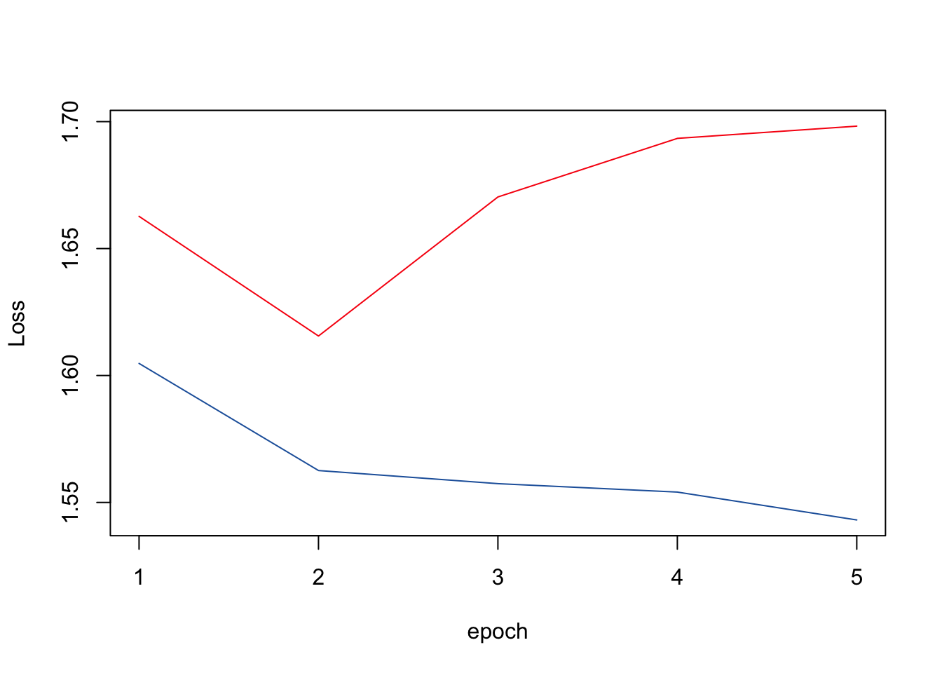
10.5 Multi-modal Neural Network
10.5.0.1 Task: CNN for the SDM dataset
The next exercise is based on the SDM dataset
Follow the steps above and build your own convolutional neural network.
Finally, submit your predictions to the submission server. If you have extra time, take a look at kaggle and find the SDM dataset challenge for specific architectures tailored for this dataset.
Hint: Take a look at the loss_binary_focal_crossentropy function from the keras package!
Prepare data:
load("sdm.RData")

# Preparation of images
train = sdm_img$train/max(sdm_img$train, sdm_img$test, na.rm = TRUE)
test = sdm_img$test/max(sdm_img$test, sdm_img$test, na.rm = TRUE)
train[is.na(train)] = 0
test[is.na(test)] = 0
train = aperm(train, c(1, 3, 4, 2))
test = aperm(test, c(1, 3, 4, 2))

labels = Y_train

# torch / cito -> channels must be at the second dim
train_torch = aperm(train, c(1, 4, 2, 3))
test_torch = aperm(test, c(1, 4, 2, 3))


# Preparation of env data
trainX = sdm_env$train
testX = sdm_env$test

trainX = missRanger::missRanger(trainX, num.trees = 50L)
Missing value imputation by random forests
Skip constant features for imputation:  HumanFootprint-greenhouse, HumanFootprint-harbour, HumanFootprint-dump-site
Variables to impute:        Elevation, Soilgrid-cec, Soilgrid-cfvo, Soilgrid-clay, Soilgrid-nitrogen, Soilgrid-phh2o, Soilgrid-sand, Soilgrid-silt, Soilgrid-bdod, Soilgrid-soc
Variables used to impute:   surveyId, Bio1, Bio2, Bio3, Bio4, Bio5, Bio6, Bio7, Bio8, Bio9, Bio10, Bio11, Bio12, Bio13, Bio14, Bio15, Bio16, Bio17, Bio18, Bio19, Soilgrid-bdod, Soilgrid-cec, Soilgrid-cfvo, Soilgrid-clay, Soilgrid-nitrogen, Soilgrid-phh2o, Soilgrid-sand, Soilgrid-silt, Soilgrid-soc, Elevation, LandCover-1, LandCover-2, LandCover-3, LandCover-4, LandCover-5, LandCover-6, LandCover-7, LandCover-8, LandCover-9, LandCover-10, LandCover-11, LandCover-12, LandCover-13, HumanFootprint-cemetery, HumanFootprint-reservoir, HumanFootprint-farmland, HumanFootprint-building-copernicus, HumanFootprint-forest, HumanFootprint-building-residential, HumanFootprint-building-commercial, HumanFootprint-grass, HumanFootprint-quarry, HumanFootprint-road, HumanFootprint-salt, HumanFootprint-building-industrial, HumanFootprint-vineyard, HumanFootprint-military, HumanFootprint-construction-site, HumanFootprint-orchard, HumanFootprint-meadow, HumanFootprint-farmyard, HumanFootprint-railway, community

iter 1

  |
  |                                                                      |   0%
  |
  |=======                                                               |  10%
  |
  |==============                                                        |  20%
  |
  |=====================                                                 |  30%
  |
  |============================                                          |  40%
  |
  |===================================                                   |  50%
  |
  |==========================================                            |  60%
  |
  |=================================================                     |  70%
  |
  |========================================================              |  80%
  |
  |===============================================================       |  90%
  |
  |======================================================================| 100%
iter 2

  |
  |                                                                      |   0%
  |
  |=======                                                               |  10%
  |
  |==============                                                        |  20%
  |
  |=====================                                                 |  30%
  |
  |============================                                          |  40%
  |
  |===================================                                   |  50%
  |
  |==========================================                            |  60%
  |
  |=================================================                     |  70%
  |
  |========================================================              |  80%
  |
  |===============================================================       |  90%
  |
  |======================================================================| 100%
iter 3

  |
  |                                                                      |   0%
  |
  |=======                                                               |  10%
  |
  |==============                                                        |  20%
  |
  |=====================                                                 |  30%
  |
  |============================                                          |  40%
  |
  |===================================                                   |  50%
  |
  |==========================================                            |  60%
  |
  |=================================================                     |  70%
  |
  |========================================================              |  80%
  |
  |===============================================================       |  90%
  |
  |======================================================================| 100%
iter 4

  |
  |                                                                      |   0%
  |
  |=======                                                               |  10%
  |
  |==============                                                        |  20%
  |
  |=====================                                                 |  30%
  |
  |============================                                          |  40%
  |
  |===================================                                   |  50%
  |
  |==========================================                            |  60%
  |
  |=================================================                     |  70%
  |
  |========================================================              |  80%
  |
  |===============================================================       |  90%
  |
  |======================================================================| 100%
testX = missRanger::missRanger(testX, num.trees = 50L)Missing value imputation by random forests
Skip constant features for imputation:  HumanFootprint-greenhouse, HumanFootprint-harbour, HumanFootprint-salt, HumanFootprint-military, HumanFootprint-dump-site
Variables to impute:        Soilgrid-bdod, Soilgrid-soc, Soilgrid-cec, Soilgrid-cfvo, Soilgrid-clay, Soilgrid-nitrogen, Soilgrid-phh2o, Soilgrid-sand, Soilgrid-silt
Variables used to impute:   surveyId, Bio1, Bio2, Bio3, Bio4, Bio5, Bio6, Bio7, Bio8, Bio9, Bio10, Bio11, Bio12, Bio13, Bio14, Bio15, Bio16, Bio17, Bio18, Bio19, Soilgrid-bdod, Soilgrid-cec, Soilgrid-cfvo, Soilgrid-clay, Soilgrid-nitrogen, Soilgrid-phh2o, Soilgrid-sand, Soilgrid-silt, Soilgrid-soc, Elevation, LandCover-1, LandCover-2, LandCover-3, LandCover-4, LandCover-5, LandCover-6, LandCover-7, LandCover-8, LandCover-9, LandCover-10, LandCover-11, LandCover-12, LandCover-13, HumanFootprint-cemetery, HumanFootprint-reservoir, HumanFootprint-farmland, HumanFootprint-building-copernicus, HumanFootprint-forest, HumanFootprint-building-residential, HumanFootprint-building-commercial, HumanFootprint-grass, HumanFootprint-quarry, HumanFootprint-road, HumanFootprint-building-industrial, HumanFootprint-vineyard, HumanFootprint-construction-site, HumanFootprint-orchard, HumanFootprint-meadow, HumanFootprint-farmyard, HumanFootprint-railway, community

iter 1

  |
  |                                                                      |   0%
  |
  |========                                                              |  11%
  |
  |================                                                      |  22%
  |
  |=======================                                               |  33%
  |
  |===============================                                       |  44%
  |
  |=======================================                               |  56%
  |
  |===============================================                       |  67%
  |
  |======================================================                |  78%
  |
  |==============================================================        |  89%
  |
  |======================================================================| 100%
iter 2

  |
  |                                                                      |   0%
  |
  |========                                                              |  11%
  |
  |================                                                      |  22%
  |
  |=======================                                               |  33%
  |
  |===============================                                       |  44%
  |
  |=======================================                               |  56%
  |
  |===============================================                       |  67%
  |
  |======================================================                |  78%
  |
  |==============================================================        |  89%
  |
  |======================================================================| 100%
iter 3

  |
  |                                                                      |   0%
  |
  |========                                                              |  11%
  |
  |================                                                      |  22%
  |
  |=======================                                               |  33%
  |
  |===============================                                       |  44%
  |
  |=======================================                               |  56%
  |
  |===============================================                       |  67%
  |
  |======================================================                |  78%
  |
  |==============================================================        |  89%
  |
  |======================================================================| 100%
human_footprint = rowSums(trainX[,44:65])
landcover = rowSums(trainX[,31:43])
trainX = trainX[,2:30]
trainX$human_footprint = human_footprint
trainX$landcover = landcover
human_footprint = rowSums(testX[,44:65])
landcover = rowSums(testX[,31:43])
testX = testX[,2:30]
testX$human_footprint = human_footprint
testX$landcover = landcover
trainXs = scale(trainX)
testXs = scale(testX)
colnames(trainXs) = stringr::str_remove(colnames(trainXs), "-")
colnames(trainXs) = stringr::str_remove(colnames(trainXs), "-")
colnames(testXs) = colnames(trainXs)Tip: Take a look at the dataset chapter.
Build model:
net = nn_module(
  "mmn",
  initialize = function(dropout_rate = 0.3){

    # CNN
    self$conv1 = nn_conv2d(4, 8L, 4L)
    self$dropout1 = nn_dropout2d(p = dropout_rate)
    self$fc1 = nn_linear(1800, 50L)

    # Env dnn
    self$h1 = nn_linear(ncol(trainXs), 50L)
    self$h2 = nn_linear(50L, 50L)

    # fusion network
    self$f1 = nn_linear(100L, 50L)
    self$f2 = nn_linear(50L, ncol(labels))
  },
  forward = function(img, env){
    path_img =
      img |>
        self$conv1() |>
        nnf_relu() |>
        self$dropout1() |>
        nnf_max_pool2d(4) |>
        torch_flatten(start_dim = 2) |>
        self$fc1() |>
        nnf_relu()

    path_env =
      env |>
      self$h1() |>
      nnf_relu() |>
      self$h2() |>
      nnf_relu()

    # combine
    comb = torch_cat(list(path_img, path_env), dim = 2L)
    comb |>
      self$f1() |>
      nnf_relu() |>
      self$f2() |>
      nnf_sigmoid()
  }
)

model_torch = net()
opt = optim_adam(params = model_torch$parameters, lr = 0.01)

dataset = tensor_dataset(torch_tensor(train_torch),
                         torch_tensor(trainXs),
                         torch_tensor(labels, dtype = torch_float())
                         )
train_dl = torch::dataloader(dataset, batch_size = 50L, shuffle = TRUE)

for(e in 1:3){
  losses = c()
  coro::loop(
    for(batch in train_dl){
      opt$zero_grad()
      pred = model_torch(batch[[1]], batch[[2]])
      loss = nnf_binary_cross_entropy(pred, batch[[3]], reduction = "mean")
      loss$backward()
      opt$step()
      losses = c(losses, loss$item())
    }
  )
  cat(sprintf("Loss at epoch %d: %3f\n", e, mean(losses)))
}
Loss at epoch 1: 0.125722
Loss at epoch 2: 0.099738
Loss at epoch 3: 0.096652Predictions:
# Prediction on training data:
model_torch$eval()
predictions = model_torch(torch_tensor(train_torch), torch_tensor(trainXs))  |> as_array()

aucs = sapply(1:ncol(Y_train), function(i) Metrics::auc(Y_train[,i], predictions[,i]))
mean(aucs)
[1] 0.8645947predictions = model_torch(torch_tensor(test_torch), torch_tensor(testXs)) |> as_array()
write.csv(data.frame(y = as.vector(predictions)), file = "cnn.csv")architecture = create_architecture(
conv(n_kernels = 8L, kernel_size = 2L, activation = "relu"),
maxPool(),
default_dropout = 0.2
)
model.cito = mmn(labels~
cnn(X=cnn_data, architecture = architecture) +
dnn(~., data = dnn_data),
dataList = list(labels = labels, cnn_data=train_torch, dnn_data=trainXs),
loss = "bernoulli",
batchsize = 128L,
epochs = 5L,
validation = 0.0,
optimizer = "adam",
lr = 0.001)Loss at epoch 1: 0.250511, lr: 0.00100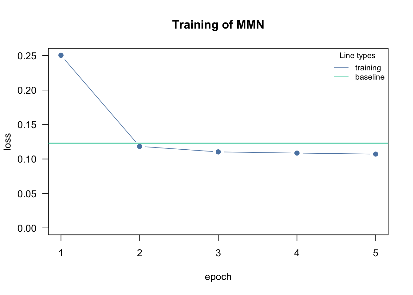
Loss at epoch 2: 0.118297, lr: 0.00100
Loss at epoch 3: 0.110314, lr: 0.00100
Loss at epoch 4: 0.108605, lr: 0.00100
Loss at epoch 5: 0.107127, lr: 0.00100
predictions = model.cito |> predict(newdata = list(cnn_data=train_torch, dnn_data=trainXs))
aucs = sapply(1:ncol(Y_train), function(i) Metrics::auc(Y_train[,i], predictions[,i]))
mean(aucs)[1] 0.7708853Submission:
predictions = model.cito |> predict(newdata = list(cnn_data=test_torch, dnn_data=testXs))
write.csv(data.frame(y = as.vector(predictions)), file = "cnn.csv")