devtools::install_github(repo = "florianhartig/EcoData", subdir = "EcoData",
dependencies = TRUE, build_vignettes = FALSE)Appendix A — Datasets
You can download the data sets we use in the course here (ignore browser warnings) or by installing the EcoData package:
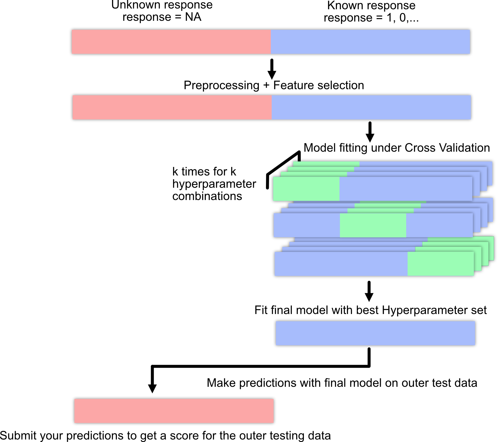
A.1 Machine learning pipeline / workflow
A.2 Titanic
The data set is a collection of Titanic passengers with information about their age, class, sex, and their survival status. The competition is simple here: Train a machine learning model and predict the survival probability.
The Titanic data set is very well explored and serves as a stepping stone in many machine learning careers. For inspiration and data exploration notebooks, check out this kaggle competition.
Response variable: “survived”
A minimal working example:
- Load data set:
library(EcoData)

data(titanic_ml)
titanic = titanic_ml
summary(titanic)
pclass survived name sex
Min. :1.000 Min. :0.0000 Length :1309 female:466
1st Qu.:2.000 1st Qu.:0.0000 N.unique :1307 male :843
Median :3.000 Median :0.0000 N.blank : 0
Mean :2.295 Mean :0.3853 Min.nchar: 12
3rd Qu.:3.000 3rd Qu.:1.0000 Max.nchar: 82
Max. :3.000 Max. :1.0000
NAs :655
age sibsp parch ticket
Min. : 0.1667 Min. :0.0000 Min. :0.000 CA. 2343: 11
1st Qu.:21.0000 1st Qu.:0.0000 1st Qu.:0.000 1601 : 8
Median :28.0000 Median :0.0000 Median :0.000 CA 2144 : 8
Mean :29.8811 Mean :0.4989 Mean :0.385 3101295 : 7
3rd Qu.:39.0000 3rd Qu.:1.0000 3rd Qu.:0.000 347077 : 7
Max. :80.0000 Max. :8.0000 Max. :9.000 347082 : 7
NAs :263 (Other) :1261
fare cabin embarked body
Min. : 0.000 :1014 : 2 Min. : 1.0
1st Qu.: 7.896 C23 C25 C27 : 6 C:270 1st Qu.: 72.0
Median : 14.454 B57 B59 B63 B66: 5 Q:123 Median :155.0
Mean : 33.295 G6 : 5 S:914 Mean :160.8
3rd Qu.: 31.275 B96 B98 : 4 3rd Qu.:256.0
Max. :512.329 C22 C26 : 4 Max. :328.0
NAs :1 (Other) : 271 NAs :1188
home.dest
:564
New York, NY : 64
London : 14
Montreal, PQ : 10
Cornwall / Akron, OH: 9
Paris, France : 9
(Other) :639 - Impute missing values (not our response variable!):
library(missRanger)
library(dplyr)
set.seed(123)

titanic_imputed = titanic |> select(!any_of(c("name", "ticket", "cabin", "boat", "home.dest")))
titanic_imputed = missRanger::missRanger(data = titanic_imputed |>
                                           select(-survived), verbose = 0)
titanic_imputed$survived = titanic$survived- Split into training and test set:
train = titanic_imputed[!is.na(titanic$survived), ]
test = titanic_imputed[is.na(titanic$survived), ]- Train model:
model = glm(survived~., data = train, family = binomial())- Predictions:
preds = predict(model, data = test, type = "response")
head(preds)
561 321 1177 1098 1252 1170
0.7857118 0.3509419 0.0157811 0.1181712 0.1367818 0.1132234 - Create submission csv:
write.csv(data.frame(y = preds), file = "glm.csv")And submit the csv on http://132.199.73.15:8500.
A.3 Plant-pollinator Database
The plant-pollinator database is a collection of plant-pollinator interactions with traits for plants and pollinators. The idea is pollinators interact with plants when their traits fit (e.g. the tongue of a bee needs to match the shape of a flower). We explored the advantage of machine learning algorithms over traditional statistical models in predicting species interactions in our paper. If you are interested you can have a look here.
Response variable: “interaction”
A minimal working example:
- Load data set:
library(EcoData)

data(plantPollinator_df)
plant_poll = plantPollinator_df
summary(plant_poll)
crop insect type
Vaccinium_corymbosum: 256 Andrena_wilkella : 80 Length :20480
Brassica_napus : 256 Andrena_barbilabris: 80 N.unique : 2
Carum_carvi : 256 Andrena_cineraria : 80 N.blank : 0
Coriandrum_sativum : 256 Andrena_flavipes : 80 Min.nchar: 9
Daucus_carota : 256 Andrena_gravida : 80 Max.nchar: 10
Malus_domestica : 256 Andrena_haemorrhoa : 80
(Other) :18944 (Other) :20000
season diameter corolla colour
Length :20480 Min. : 2.00 Length :20480 Length :20480
N.unique : 11 1st Qu.: 5.00 N.unique : 3 N.unique : 7
N.blank : 0 Median : 19.00 N.blank : 0 N.blank : 0
Min.nchar: 4 Mean : 27.03 Min.nchar: 4 Min.nchar: 3
Max.nchar: 8 3rd Qu.: 25.00 Max.nchar: 11 Max.nchar: 6
NAs : 1024 Max. :150.00 NAs : 256 NAs : 256
NAs :9472
nectar b.system s.pollination inflorescence
Length :20480 Length :20480 Length :20480 Length :20480
N.unique : 2 N.unique : 4 N.unique : 2 N.unique : 4
N.blank : 0 N.blank : 0 N.blank : 0 N.blank : 0
Min.nchar: 2 Min.nchar: 7 Min.nchar: 2 Min.nchar: 3
Max.nchar: 3 Max.nchar: 13 Max.nchar: 3 Max.nchar: 17
NAs : 1024
composite guild tongue body
Length :20480 Length :20480 Min. : 2.000 Min. : 2.00
N.unique : 2 N.unique : 14 1st Qu.: 4.800 1st Qu.: 8.00
N.blank : 0 N.blank : 0 Median : 6.600 Median :10.50
Min.nchar: 2 Min.nchar: 5 Mean : 8.104 Mean :10.66
Max.nchar: 3 Max.nchar: 14 3rd Qu.:10.500 3rd Qu.:13.00
Max. :26.400 Max. :25.00
NAs :17040 NAs :6160
sociality feeding interaction
Length :20480 Length :20480 0 :14095
N.unique : 2 N.unique : 3 1 : 595
N.blank : 0 N.blank : 0 NAs: 5790
Min.nchar: 2 Min.nchar: 9
Max.nchar: 3 Max.nchar: 11
NAs : 960 NAs : 2160
- Impute missing values (not our response variable!) We will select only a few predictors here (you can work with all predictors of course).
library(missRanger)
library(dplyr)
set.seed(123)

plant_poll_imputed = plant_poll |> select(diameter,
                                           corolla,
                                           tongue,
                                           body,
                                           interaction)
plant_poll_imputed = missRanger::missRanger(data = plant_poll_imputed |>
                                              select(-interaction), verbose = 0)
plant_poll_imputed$interaction = plant_poll$interaction- Split into training and test set:
train = plant_poll_imputed[!is.na(plant_poll_imputed$interaction), ]
test = plant_poll_imputed[is.na(plant_poll_imputed$interaction), ]- Train model:
model = glm(interaction~., data = train, family = binomial())- Predictions:
preds = predict(model, newdata = test, type = "response")
head(preds)
1 2 3 4 5 6
0.03006681 0.04649644 0.04113120 0.04113120 0.02990536 0.03987069 - Create submission csv:
write.csv(data.frame(y = preds), file = "glm.csv")A.4 Species distribution modeling (SDM)
This data set is based on the GeoLifeCLEF 2025 challenge and poses a multi-species distribution modeling task: for a set of geographic sites (which we call communities), predict which of 448 plant species are present, using environmental predictors that describe each site. Unlike the other data sets, the response is not a single column but a presence-absence matrix — one binary label per species for every community.
Response variable: presence/absence of each of the 448 species (a community \(\times\) species matrix).
Predictors: environmental variables characterizing each community — e.g. bioclimatic variables (Bio1–Bio19, such as mean annual temperature and precipitation), soil properties (e.g. SoilGrids pH), elevation, and similar geographic layers.
A.4.1 Data structure
For both the training and test communities you get two tables:
- an environmental table (
env_df) — one row per community, one column per environmental predictor; - a presence-absence label table (
labels) — a community \(\times\) species matrix of 0/1, with species in the columns (namedsp_9,sp_53,sp_96, …).
The test set contains 2000 communities and 448 species. The labels of the test communities are withheld — those are what you predict and submit.
The same data is also available in long format, which is often more convenient for modeling. In long format there is one row per community \(\times\) species combination, with the columns community, species, present (0/1), plus the environmental predictors of that community repeated across its species:
community  species  present  Bio1  Bio2  ...  Elevation
   212      sp_3       1      ...   ...        ...
   212      sp_7       0      ...   ...        ...
Wide and long are two views of the same data; you can always convert between them. For example, to turn a long label table back into the wide matrix:
load("sdm.RData")

library(missRanger)
library(tidyverse)

sdm_long |> summary()

sdm_long[,-3] = sdm_long[,-3]  |>  mutate(across(everything(), ~ifelse(is.na(.), mean(., na.rm = TRUE), .)))

train = sdm_long[!is.na(sdm_long$present), ]
test = sdm_long[is.na(sdm_long$present), ]

# sub sample training data due to computational constraints
indices = sample.int(nrow(train), 5000)
train$present = as.factor(train$present)
A.4.2 A minimal working example
Dataset can be downloaded from the submission server or from dropbox
There are two natural modeling strategies:
- Long format + a single binary classifier with the species included as a predictor (e.g. a random forest or DNN on the long table). This gives a presence probability for every community \(\times\) species row directly.
- Wide format + a multi-output model that predicts the full 2000 \(\times\) 448 matrix at once.
A simple example using the long table:
library(ranger)
set.seed(123)

rf = ranger(present ~ ., data = train[indices, -c(1, 4)], # without community and survey ID
            classification = TRUE, probability = TRUE, num.trees = 100L) # only 100 trees to speed up the predictions of the test dataset

# presence probability per community x species row:
preds = predict(rf, data = test)$predictions[, 2]
A.4.3 Submission format — long or wide
You can submit your predictions in either format; the leaderboard accepts both.
Long — the 896,000 (= 2000 \(\times\) 448) probabilities stacked into a single column. The scorer rebuilds the matrix with matrix(y, nrow = 2000), which fills it column-by-column, so the values must be ordered all 2000 communities of species 1, then all of species 2, … — exactly what as.vector() of the wide matrix produces:
write.csv(data.frame(y = as.vector(preds)),
          file = "sdm.csv", row.names = FALSE)
Wide — a 2000 \(\times\) 448 matrix of presence probabilities, communities in rows and species in columns, in the same species order as the label matrix (sp_9, sp_53, …):
write.csv(pred_matrix, file = "sdm.csv", row.names = FALSE)Two checks before uploading: dim(pred_matrix) should be 2000 x 448, and the saved file should have either 448 value columns (wide) or 896,000 rows (long). If you build the long vector directly from a long-format prediction (like the random forest above), make sure its rows are in community-within-species order, so the reshape lines up with the species columns of the label matrix — otherwise the values misalign and the score collapses.
Evaluation metric: submissions are scored with a weighted AUC — the mean of the per-species AUC values, weighted so that rare species count more than common ones.
Then submit the csv on http://132.199.73.15:8500.
A.5 Flower
A collection of over 4000 flower images of 5 plant species. The data set is from kaggle but we downsampled the images from \(320*240\) to \(80*80\) pixels. You can a) download the data set here or b) get it via the EcoData package.
Notes:
- Check out convolutional neural network notebooks on kaggle (they are often written in Python but you can still copy the architectures), e.g. this one.
- Last year’s winners have used a transfer learning approach (they achieved around 70% accuracy), check out this notebook, see also the section about transfer learning @ref(transfer).
Response variable: “Plant species”
- Load data set:
library(tensorflow)
library(keras3)

train = EcoData::dataset_flower()$train/255
test = EcoData::dataset_flower()$test/255
labels = EcoData::dataset_flower()$labels
Let’s visualize a flower:
train[100,,,] |>
  image_to_array() |>
  as.raster() |>
  plot()
- Build and train model:
model = keras_model_sequential()
model |>
  layer_conv_2d(filters = 4L, kernel_size = 2L,
                input_shape = list(80L, 80L, 3L)) |>
  layer_max_pooling_2d() |>
  layer_flatten() |>
  layer_dense(units = 5L, activation = "softmax")

### Model fitting ###

model |>
  compile(loss = loss_categorical_crossentropy,
          optimizer = optimizer_adamax(learning_rate = 0.01))

model |>
fit(x = train, y = keras::k_one_hot(labels, 5L))- Predictions:
# Prediction on training data:
pred = apply(model |> predict(train), 1, which.max)
Metrics::accuracy(pred - 1L, labels)
table(pred)

# Prediction for the submission server:
pred = model |> predict(test) |> apply(1, which.max) - 1L
table(pred)- Create submission csv:
write.csv(data.frame(y = pred), file = "cnn.csv")