xAI aims at explaining how predictions are being made. In general, xAI != causality. xAI methods measure which variables are used for predictions by the algorithm, or how far variables improve predictions. The important point to note here: If a variable causes something, we could also expect that it helps predicting the very thing. The opposite, however, is not generally true - very often it is possible that a variable that doesn’t cause anything can predict something.
In statistics courses (in particular our course: Advanced Biostatistics), we discuss the issue of causality at full length. Here, we don’t want to go into the details, but again, you should in general resist to interpret indicators of importance in xAI as causal effects. They tell you something about what’s going on in the algorithm, not about what’s going on in reality.
9.1 Causal Inference on Static Data
Methods for causal inference depend on whether we have dynamic or static data. The latter is the more common case. With static data, the problem is confounding. If you have several correlated predictors, you can get spurious correlations between a given predictor and the response, although there is no causal effect in general.
Multiple regression and few other methods are able to correct for other predictors and thus isolate the causal effect. The same is not necessarily true for machine learning algorithms and xAI methods. This is not a bug, but a feature - for making good predictions, it is often no problem, but rather an advantage to also use non-causal predictors.
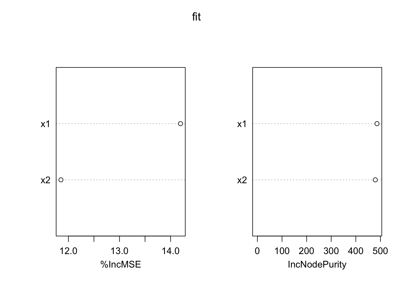
Here an example for the indicators of variable importance in the random forest algorithm. The purpose of this script is to show that random forest variable importance will split importance values for collinear variables evenly, even if collinearity is low enough so that variables are separable and would be correctly separated by an lm / ANOVA.
We first simulate a data set with 2 predictors that are strongly correlated, but only one of them has an effect on the response.
library(randomForest)
randomForest 4.7-1.2
Type rfNews() to see new features/changes/bug fixes.
set.seed(123)# Simulation parameters.n =1000col =0.7# Create collinear predictors.x1 =runif(n)x2 = col * x1 + (1-col) *runif(n)# Response is only influenced by x1.y = x1 +rnorm(n)
lm / anova correctly identify \(x1\) as causal variable.
summary(lm(y ~ x1 + x2))
Call:
lm(formula = y ~ x1 + x2)

Residuals:
    Min      1Q  Median      3Q     Max
-3.0709 -0.6939  0.0102  0.6976  3.3373

Coefficients:
            Estimate Std. Error t value Pr(>|t|)
(Intercept)  0.02837    0.08705   0.326 0.744536
x1           1.07383    0.27819   3.860 0.000121 ***
x2          -0.04547    0.37370  -0.122 0.903186
---
Signif. codes:  0 '***' 0.001 '**' 0.01 '*' 0.05 '.' 0.1 ' ' 1

Residual standard error: 1.011 on 997 degrees of freedom
Multiple R-squared:  0.08104,   Adjusted R-squared:  0.0792
F-statistic: 43.96 on 2 and 997 DF,  p-value: < 2.2e-16
How the random forest works - variables are randomly hidden from the regression tree when the trees for the forest are built.
Remember that as \(x1 \propto x2\), we can use \(x2\) as a replacement for \(x1\).
Remember that the variable importance measures the average contributions of the different variables in the trees of the forest.
Note
We found that (D)NN can better separate collinearity than the other classical ML algorithms. Probably, this is one of the advantages of (D)NN over RF or BRT for tabular data for two reasons:
We can trust DNN more “causally” than the other algorithms, in the sense that an effect in the DNN is not just a consequence of collinearity.
Causality (or the ability to correctly estimate causal effects) is important for predicting out-of-distribution, e.g., changing collinearity structures
library(cito)nn.fit =dnn(y~x1+x2, loss ="mse", data =data.frame(y = y, x1=x1, x2=x2), verbose = F, plot = F)
Registered S3 methods overwritten by 'reformulas':
  method       from
  head.call    cito
  head.formula cito
  head.name    cito
summary(nn.fit)
Summary of Deep Neural Network Model

Feature Importance:
  variable importance_1
1       x1   0.13864303
2       x2   0.00346932

Average Conditional Effects:
   Response_1
x1  0.9445299
x2  0.1204029

Standard Deviation of Conditional Effects:
   Response_1
x1 0.04281256
x2 0.06451134
9.2 Automatic Causal Discovery
But how to get the causal graph? In statistics, it is common to “guess” it and afterwards do residual checks, in the same way as we guess the structure of a regression. For more complicated problems, however, this is unsatisfying. Some groups therefore work on so-called causal discovery algorithms, i.e. algorithms that automatically generate causal graphs from data. One of the most classic algorithms of this sort is the PC algorithm. Here an example using the pcalg package:
library(pcalg)
Loading the data:
data("gmG", package ="pcalg") # Loads data sets gmG and gmG8.suffStat =list(C =cor(gmG8$x), n =nrow(gmG8$x))varNames = gmG8$g@nodes
First, the skeleton algorithm creates a basic graph without connections (a skeleton of the graph).
What is missing here is the direction of the errors. The PC algorithm now makes tests for conditional independence, which allows fixing a part (but typically not all) of the directions of the causal arrows.
When working with dynamic data, we can use an additional piece of information - the cause usually precedes the effect, which means that we can test for a time-lag between cause and effect to determine the direction of causality. This way of testing for causality is known as Granger causality, or Granger methods. Here an example:
library(lmtest)## What came first: the chicken or the egg?data(ChickEgg)grangertest(egg ~ chicken, order =3, data = ChickEgg)
Granger causality test

Model 1: egg ~ Lags(egg, 1:3) + Lags(chicken, 1:3)
Model 2: egg ~ Lags(egg, 1:3)
  Res.Df Df      F Pr(>F)
1     44
2     47 -3 0.5916 0.6238
grangertest(chicken ~ egg, order =3, data = ChickEgg)
As we have seen, there are already a few methods / algorithms for discovering causality from large data sets, but the systematic transfer of these concepts to machine learning, in particular deep learning, is still at its infancy. At the moment, this field is actively researched and changes extremely fast, so we recommend using Google to see what is currently going on. Particular in business and industry, there is a large interest in learning about causal effect from large data sets. In our opinion, a great topic for young scientists to specialize on.