As we have seen today, many of the machine learning algorithms are distributed over several packages but the general machine learning pipeline is very similar for all models: feature engineering, feature selection, hyperparameter tuning and cross-validation.
Machine learning frameworks such as mlr3 or tidymodels provide a general interface for the ML pipeline, in particular the training and the hyperparameter tuning with nested CV. They support most ML packages/algorithms.
C.1 mlr3
The key features of mlr3 are:
All common machine learning packages are integrated into mlr3, you can easily switch between different machine learning algorithms.
A common ‘language’/workflow to specify machine learning pipelines.
Support for different cross-validation strategies.
Hyperparameter tuning for all supported machine learning algorithms.
The mlr3 package actually consists of several packages for different tasks (e.g. mlr3tuning for hyperparameter tuning, mlr3pipelines for data preparation pipes). But let’s start with the basic workflow:
'data.frame':   4687 obs. of  40 variables:
 $ Neo.Reference.ID            : int  3449084 3702322 3406893 NA 2363305 3017307 2438430 3653917 3519490 2066391 ...
 $ Name                        : int  NA 3702322 3406893 3082923 2363305 3017307 2438430 3653917 3519490 NA ...
 $ Absolute.Magnitude          : num  18.7 22.1 24.8 21.6 21.4 18.2 20 21 20.9 16.5 ...
 $ Est.Dia.in.KM.min.          : num  0.4837 0.1011 0.0291 0.1272 0.1395 ...
 $ Est.Dia.in.KM.max.          : num  1.0815 0.226 0.0652 0.2845 0.3119 ...
 $ Est.Dia.in.M.min.           : num  483.7 NA 29.1 127.2 139.5 ...
 $ Est.Dia.in.M.max.           : num  1081.5 226 65.2 284.5 311.9 ...
 $ Est.Dia.in.Miles.min.       : num  0.3005 0.0628 NA 0.0791 0.0867 ...
 $ Est.Dia.in.Miles.max.       : num  0.672 0.1404 0.0405 0.1768 0.1938 ...
 $ Est.Dia.in.Feet.min.        : num  1586.9 331.5 95.6 417.4 457.7 ...
 $ Est.Dia.in.Feet.max.        : num  3548 741 214 933 1023 ...
 $ Close.Approach.Date         : Factor w/ 777 levels "1995-01-01","1995-01-08",..: 511 712 472 239 273 145 428 694 87 732 ...
 $ Epoch.Date.Close.Approach   : num  NA 1.42e+12 1.21e+12 1.00e+12 1.03e+12 ...
 $ Relative.Velocity.km.per.sec: num  11.22 13.57 5.75 13.84 4.61 ...
 $ Relative.Velocity.km.per.hr : num  40404 48867 20718 49821 16583 ...
 $ Miles.per.hour              : num  25105 30364 12873 30957 10304 ...
 $ Miss.Dist..Astronomical.    : num  NA 0.0671 0.013 0.0583 0.0381 ...
 $ Miss.Dist..lunar.           : num  112.7 26.1 NA 22.7 14.8 ...
 $ Miss.Dist..kilometers.      : num  43348668 10030753 1949933 NA 5694558 ...
 $ Miss.Dist..miles.           : num  26935614 6232821 1211632 5418692 3538434 ...
 $ Orbiting.Body               : Factor w/ 1 level "Earth": 1 1 1 1 1 1 1 1 1 1 ...
 $ Orbit.ID                    : int  NA 8 12 12 91 NA 24 NA NA 212 ...
 $ Orbit.Determination.Date    : Factor w/ 2680 levels "2014-06-13 15:20:44",..: 69 NA 1377 1774 2275 2554 1919 731 1178 2520 ...
 $ Orbit.Uncertainity          : int  0 8 6 0 0 0 1 1 1 0 ...
 $ Minimum.Orbit.Intersection  : num  NA 0.05594 0.00553 NA 0.0281 ...
 $ Jupiter.Tisserand.Invariant : num  5.58 3.61 4.44 5.5 NA ...
 $ Epoch.Osculation            : num  2457800 2457010 NA 2458000 2458000 ...
 $ Eccentricity                : num  0.276 0.57 0.344 0.255 0.22 ...
 $ Semi.Major.Axis             : num  1.1 NA 1.52 1.11 1.24 ...
 $ Inclination                 : num  20.06 4.39 5.44 23.9 3.5 ...
 $ Asc.Node.Longitude          : num  29.85 1.42 170.68 356.18 183.34 ...
 $ Orbital.Period              : num  419 1040 682 427 503 ...
 $ Perihelion.Distance         : num  0.794 0.864 0.994 0.828 0.965 ...
 $ Perihelion.Arg              : num  41.8 359.3 350 268.2 179.2 ...
 $ Aphelion.Dist               : num  1.4 3.15 2.04 1.39 1.51 ...
 $ Perihelion.Time             : num  2457736 2456941 2457937 NA 2458070 ...
 $ Mean.Anomaly                : num  55.1 NA NA 297.4 310.5 ...
 $ Mean.Motion                 : num  0.859 0.346 0.528 0.843 0.716 ...
 $ Equinox                     : Factor w/ 1 level "J2000": 1 1 NA 1 1 1 1 1 1 1 ...
 $ Hazardous                   : int  0 0 0 1 1 0 0 0 1 1 ...
Let’s drop time, name and ID variable and create a classification task:
data = nasa |>select(-Orbit.Determination.Date,-Close.Approach.Date, -Name, -Neo.Reference.ID)data$Hazardous =as.factor(data$Hazardous)# Create a classification task.task = TaskClassif$new(id ="nasa", backend = data,target ="Hazardous", positive ="1")
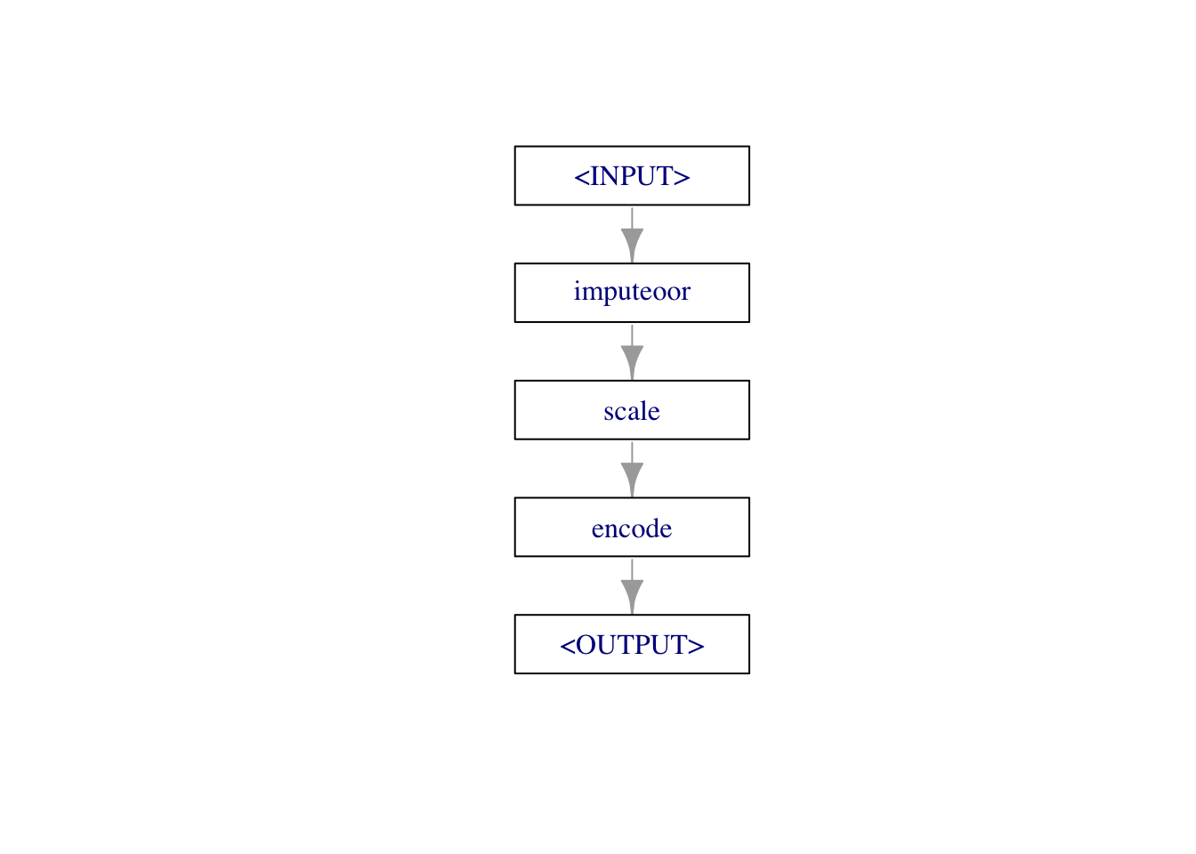
Create a generic pipeline of data transformation (imputation \(\rightarrow\) scaling \(\rightarrow\) encoding of categorical variables):
set.seed(123)# Let's create the preprocessing graph.preprocessing =po("imputeoor") %>>%po("scale") %>>%po("encode") # Run the task.transformed_task = preprocessing$train(task)[[1]]transformed_task$missings()
# Exclude the rows with a missing target from the cross-validation by keeping# only the labelled rows in the 'use' role (recent mlr3 removed the 'holdout' role).transformed_task$row_roles$use = (1:nrow(data))[!is.na(data$Hazardous)]cv10 = mlr3::rsmp("cv", folds =10L)EN =lrn("classif.glmnet", predict_type ="prob")measurement =msr("classif.auc")
result = mlr3::resample(transformed_task, EN, resampling = cv10, store_models =TRUE)# Calculate the average AUC of the holdouts.result$aggregate(measurement)
Very cool! Preprocessing + 10-fold cross-validation model evaluation in a few lines of code!
Let’s create the final predictions:
# re-expose the unlabelled rows (excluded from the 'use' role for CV) before predictingtransformed_task$row_roles$use =1:nrow(data)pred =sapply(1:10, function(i) result$learners[[i]]$predict(transformed_task,row_ids = (1:nrow(data))[is.na(data$Hazardous)])$data$prob[, "1", drop =FALSE])dim(pred)predictions =apply(pred, 1, mean)
But we are still not happy with the results, let’s do some hyperparameter tuning!
C.1.2 mlr3 - Hyperparameter Tuning
With mlr3, we can easily extend the above example to do hyperparameter tuning within nested cross-validation (the tuning has its own inner cross-validation).
Print the hyperparameter space of our glmnet learner:
EN$param_set
<ParamSet(35)>
                  id    class lower upper nlevels        default  value
              <char>   <char> <num> <num>   <num>         <list> <list>
 1:            alpha ParamDbl     0     1     Inf              1 [NULL]
 2:          nlambda ParamInt     1   Inf     Inf            100 [NULL]
 3: lambda.min.ratio ParamDbl     0     1     Inf <NoDefault[0]> [NULL]
 4:           lambda ParamUty    NA    NA     Inf         [NULL] [NULL]
 5:      standardize ParamLgl    NA    NA       2           TRUE [NULL]
 6:        intercept ParamLgl    NA    NA       2           TRUE [NULL]
 7:          exclude ParamUty    NA    NA     Inf         [NULL] [NULL]
 8:   penalty.factor ParamUty    NA    NA     Inf <NoDefault[0]> [NULL]
 9:     lower.limits ParamUty    NA    NA     Inf           -Inf [NULL]
10:     upper.limits ParamUty    NA    NA     Inf            Inf [NULL]
11:    type.logistic ParamFct    NA    NA       2 <NoDefault[0]> [NULL]
12: type.multinomial ParamFct    NA    NA       2 <NoDefault[0]> [NULL]
13:            relax ParamLgl    NA    NA       2          FALSE [NULL]
14:         trace.it ParamInt     0     1       2              0 [NULL]
15:             maxp ParamInt     1   Inf     Inf <NoDefault[0]> [NULL]
16:             path ParamLgl    NA    NA       2          FALSE [NULL]
17:             fdev ParamDbl     0     1     Inf          1e-05 [NULL]
18:           devmax ParamDbl     0     1     Inf          0.999 [NULL]
19:              eps ParamDbl     0     1     Inf          1e-06 [NULL]
20:              big ParamDbl  -Inf   Inf     Inf        9.9e+35 [NULL]
21:            mnlam ParamInt     1   Inf     Inf              5 [NULL]
22:             pmin ParamDbl     0     1     Inf          1e-09 [NULL]
23:             exmx ParamDbl  -Inf   Inf     Inf            250 [NULL]
24:             prec ParamDbl  -Inf   Inf     Inf          1e-10 [NULL]
25:             mxit ParamInt     1   Inf     Inf            100 [NULL]
26:            epsnr ParamDbl     0     1     Inf          1e-06 [NULL]
27:           mxitnr ParamInt     1   Inf     Inf             25 [NULL]
28:           thresh ParamDbl     0   Inf     Inf          1e-07 [NULL]
29:            maxit ParamInt     1   Inf     Inf         100000 [NULL]
30:            dfmax ParamInt     0   Inf     Inf         [NULL] [NULL]
31:             pmax ParamInt     0   Inf     Inf         [NULL] [NULL]
32:            exact ParamLgl    NA    NA       2          FALSE [NULL]
33:                s ParamDbl     0   Inf     Inf           0.01 [NULL]
34:            gamma ParamDbl     0     1     Inf              1 [NULL]
35:  use_pred_offset ParamLgl    NA    NA       2 <NoDefault[0]>   TRUE
                  id    class lower upper nlevels        default  value
              <char>   <char> <num> <num>   <num>         <list> <list>
Define the hyperparameter space of the random forest:
Now we can wrap it normally into the 10-fold cross-validated setup as done previously:
# Calculate the average AUC of the holdouts.result$aggregate(measurement)
classif.auc
  0.6767554
Let’s create the final predictions:
# re-expose the unlabelled rows (excluded from the 'use' role for CV) before predictingtransformed_task$row_roles$use =1:nrow(data)pred =sapply(1:3, function(i) result$learners[[i]]$predict(transformed_task,row_ids = (1:nrow(data))[is.na(data$Hazardous)])$data$prob[, "1", drop =FALSE])dim(pred)predictions =apply(pred, 1, mean)
C.2 Exercises
C.2.1 Tuning Regularization
Question: Hyperparameter tuning - Titanic dataset
Tune architecture
Tune training parameters (learning rate, batch size) and regularization
Hints
cito has a feature to automatically tune hyperparameters under Cross Validation!
passing tune(...) to a hyperparameter will tell cito to tune this specific hyperparameter
the tuning = config_tuning(...) let you specify the cross-validation strategy and the number of hyperparameters that should be tested (steps = number of hyperparameter combinations that should be tried)
after tuning, cito will fit automatically a model with the best hyperparameters on the full data and will return this model
Minimal example with the iris dataset:
library(cito)df = irisdf[,1:4] =scale(df[,1:4])model_tuned =dnn(Species~., loss ="softmax",data = iris,lambda =tune(lower =0.0, upper =0.2), # you can pass the "tune" function to a hyerparametertuning =config_tuning(CV =3, steps =20L) )# tuning resultsmodel_tuned$tuning# model_tuned is now already the best model!
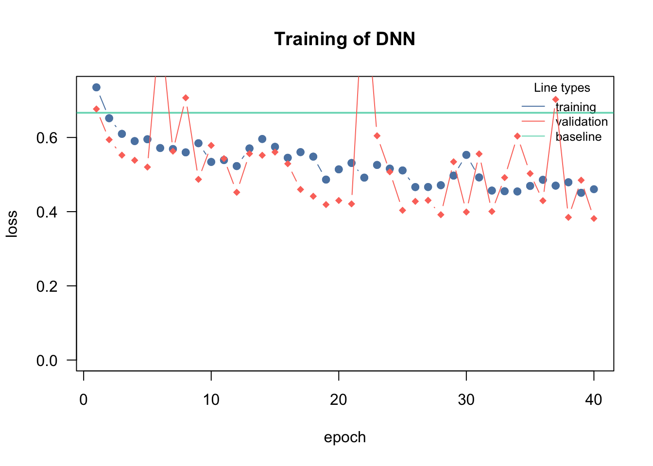
library(EcoData)library(dplyr)library(missRanger)data(titanic_ml)data = titanic_mldata = data |>select(survived, sex, age, fare, pclass)data[,-1] =missRanger(data[,-1], verbose =0)data_sub = data |>mutate(age = scales::rescale(age, c(0, 1)),fare = scales::rescale(fare, c(0, 1))) |>mutate(sex =as.integer(sex) -1L,pclass =as.integer(pclass -1L))data_new = data_sub[is.na(data_sub$survived),] # for which we want to make predictions at the enddata_obs = data_sub[!is.na(data_sub$survived),] # data with known responsedata_obs$survived =as.factor(data_obs$survived)model =dnn(survived~., hidden =c(10L, 10L), # changeactivation =c("selu", "selu"), # changeloss ="binomial", lr =0.05, #changevalidation =0.2,lambda =0.001, # changealpha =0.1, # changelr_scheduler =config_lr_scheduler("reduce_on_plateau", patience =10, factor =0.9),data = data_obs, epochs =40L, verbose =TRUE, plot=TRUE)
Loss at epoch 1: training: 0.735, validation: 0.677, lr: 0.05000
Loss at epoch 2: training: 0.652, validation: 0.594, lr: 0.05000
Loss at epoch 3: training: 0.610, validation: 0.552, lr: 0.05000
Loss at epoch 4: training: 0.590, validation: 0.538, lr: 0.05000
Loss at epoch 5: training: 0.595, validation: 0.520, lr: 0.05000
Loss at epoch 6: training: 0.572, validation: 0.907, lr: 0.05000
Loss at epoch 7: training: 0.569, validation: 0.563, lr: 0.05000
Loss at epoch 8: training: 0.560, validation: 0.707, lr: 0.05000
Loss at epoch 9: training: 0.585, validation: 0.487, lr: 0.05000
Loss at epoch 10: training: 0.534, validation: 0.579, lr: 0.05000
Loss at epoch 11: training: 0.539, validation: 0.543, lr: 0.05000
Loss at epoch 12: training: 0.523, validation: 0.452, lr: 0.05000
Loss at epoch 13: training: 0.571, validation: 0.556, lr: 0.05000
Loss at epoch 14: training: 0.596, validation: 0.552, lr: 0.05000
Loss at epoch 15: training: 0.575, validation: 0.561, lr: 0.05000
Loss at epoch 16: training: 0.545, validation: 0.529, lr: 0.05000
Loss at epoch 17: training: 0.561, validation: 0.460, lr: 0.05000
Loss at epoch 18: training: 0.548, validation: 0.442, lr: 0.05000
Loss at epoch 19: training: 0.486, validation: 0.419, lr: 0.05000
Loss at epoch 20: training: 0.514, validation: 0.430, lr: 0.05000
Loss at epoch 21: training: 0.531, validation: 0.421, lr: 0.05000
Loss at epoch 22: training: 0.492, validation: 1.037, lr: 0.05000
Loss at epoch 23: training: 0.526, validation: 0.605, lr: 0.05000
Loss at epoch 24: training: 0.516, validation: 0.507, lr: 0.05000
Loss at epoch 25: training: 0.511, validation: 0.404, lr: 0.05000
Loss at epoch 26: training: 0.466, validation: 0.428, lr: 0.05000
Loss at epoch 27: training: 0.466, validation: 0.431, lr: 0.05000
Loss at epoch 28: training: 0.471, validation: 0.392, lr: 0.05000
Loss at epoch 29: training: 0.497, validation: 0.534, lr: 0.05000
Loss at epoch 30: training: 0.553, validation: 0.399, lr: 0.05000
Loss at epoch 31: training: 0.492, validation: 0.556, lr: 0.05000
Loss at epoch 32: training: 0.457, validation: 0.401, lr: 0.05000
Loss at epoch 33: training: 0.455, validation: 0.492, lr: 0.05000
Loss at epoch 34: training: 0.454, validation: 0.604, lr: 0.05000
Loss at epoch 35: training: 0.469, validation: 0.503, lr: 0.05000
Loss at epoch 36: training: 0.486, validation: 0.430, lr: 0.05000
Loss at epoch 37: training: 0.470, validation: 0.703, lr: 0.05000
Loss at epoch 38: training: 0.479, validation: 0.385, lr: 0.05000
Loss at epoch 39: training: 0.451, validation: 0.485, lr: 0.05000
Loss at epoch 40: training: 0.461, validation: 0.382, lr: 0.05000
# Predictions:predictions =predict(model, newdata = data_new, type ="response") # change prediction type to response so that cito predicts probabilitieswrite.csv(data.frame(y = predictions[,1]), file ="Max_titanic_dnn.csv")
C.2.2 Bonus: mlr3
Task: Use mlr3 for the titanic dataset
Use mlr3 to tune glmnet for the titanic dataset using nested CV
Submit single predictions and multiple predictions
If you need help, take a look at the solution, go through it line by line and try to understand it.
Prepare data
data = titanic_ml |>select(-name, -ticket, -name, -body)data$pclass =as.factor(data$pclass)data$sex =as.factor(data$sex)data$survived =as.factor(data$survived)# Change easy things manually:data$embarked[data$embarked ==""] ="S"# Fill in "empty" values.data$embarked =droplevels(as.factor(data$embarked)) # Remove unused levels ("").data$cabin = (data$cabin !="") *1# Dummy code the availability of a cabin.data$fare[is.na(data$fare)] =mean(data$fare, na.rm =TRUE)levels(data$home.dest)[levels(data$home.dest) ==""] ="unknown"if ("boat"%in%colnames(data)) levels(data$boat)[levels(data$boat) ==""] ="none"# Create a classification task.task = TaskClassif$new(id ="titanic", backend = data,target ="survived", positive ="1")task$missings()
 survived       age     cabin  embarked      fare home.dest     parch    pclass
      655       263         0         0         0         0         0         0
      sex     sibsp
        0         0
# Let's create the preprocessing graph.preprocessing =po("imputeoor") %>>%po("scale") %>>%po("encode") # Run the task.transformed_task = preprocessing$train(task)[[1]]# Exclude the rows with a missing target from the cross-validation by keeping# only the labelled rows in the 'use' role (recent mlr3 removed the 'holdout' role).transformed_task$row_roles$use = (1:nrow(data))[!is.na(data$survived)]
Warning: from glmnet C++ code (error code -1); Convergence for 1th lambda value
not reached after maxit=100000 iterations; solutions for larger lambdas
returned
Warning in getcoef(fit, nvars, nx, vnames): an empty model has been returned;
probably a convergence issue
Warning: from glmnet C++ code (error code -1); Convergence for 1th lambda value
not reached after maxit=100000 iterations; solutions for larger lambdas
returned
Warning in getcoef(fit, nvars, nx, vnames): an empty model has been returned;
probably a convergence issue
Warning: from glmnet C++ code (error code -1); Convergence for 1th lambda value
not reached after maxit=100000 iterations; solutions for larger lambdas
returned
Warning in getcoef(fit, nvars, nx, vnames): an empty model has been returned;
probably a convergence issue
model$train(transformed_task)# the unlabelled rows were dropped from the 'use' role for training/CV;# re-expose them so we can predict on them by row idtransformed_task$row_roles$use =1:nrow(data)predictions = model$predict(transformed_task, row_ids = (1:nrow(data))[is.na(data$survived)])predictions = predictions$prob[, "1"]head(predictions)