devtools::install_github('citoverse/cito')7 Artificial Neural Networks
Artificial neural networks are biologically inspired: inputs are processed by weights at the neurons, the signals then accumulate at hidden nodes (analogous to axons), and only if the summed activation exceeds a certain threshold is the signal passed on.
IMPORTANT!!!
Install the development version of cito via
library(cito)7.1 Fitting (deep) neural networks with the cito package
Deep neural networks are currently the state of the art in unsupervised learning. Their ability to model different types of data (e.g. graphs, images) is one of the reasons for their rise in recent years. However, requires extensive (programming) knowledge of the underlying deep learning frameworks (e.g. TensorFlow or PyTorch), which we will teach you in two days. For tabular data, we can use packages like cito, which work similarly to regression functions like lm and allow us to train deep neural networks in one line of code:
library(cito)
nn.fit<- dnn(Species~., data = datasets::iris, loss = "cross-entropy", verbose = FALSE, plot = FALSE)
cito also supports many of the S3 methods that are available for statistical models, e.g. the summary function:
summary(nn.fit)Summary of Deep Neural Network Model
Feature Importance:
variable importance_1 importance_2 importance_3
1 Sepal.Length 9.905697e-07 0.007825332 0.007975580
2 Sepal.Width 1.046128e-05 0.001059770 0.001268195
3 Petal.Length 5.518517e-03 0.039701450 0.052728224
4 Petal.Width 3.861543e-05 0.012326420 0.013216395
Average Conditional Effects:
[,1] [,2] [,3]
Sepal.Length 0.001240780 0.08649288 -0.08773365
Sepal.Width 0.007292932 0.09102248 -0.09831542
Petal.Length -0.010407391 -0.16275001 0.17315741
Petal.Width -0.004870227 -0.14387218 0.14874241Variable importance can also be computed for non-tree algorithms (although it is slightly different, more on that on Thursday). The feature importance reports the importance of the features for distinguishing the three species, the average conditional effects are an approximation of the linear effects, and the standard deviation of the conditional effects is a measure of the non-linearity of these three variables.
7.2 Loss
Tasks such as regression and classification are fundamentally different; the former has continuous responses, while the latter has a discrete response. In ML algorithms, these different tasks can be represented by different loss functions (Classical ML algorithms also use loss functions but often they are automatically inferred, also neural networks are much more versatile, supporting more loss functions). Moreover, the tasks can differ even within regression or classification (e.g., in classification, we have binary classification (0 or 1) or multi-class classification (0, 1, or 2)). As a result, especially in DL, we have different specialized loss functions available for specific response types. The table below shows a list of supported loss functions in cito:
| Loss | Type | Example |
|---|---|---|
| mse (mean squared error) | Regression | Numeric values |
| mae (mean absolute error) | Regression | Numeric values, often used for skewed data |
| cross-entropy | Classification, multi-label | Species |
| cross-entropy | Classification, binary or multi-class | Survived/non-survived, Multi-species/communities |
| binomial | Classification, binary or multi-class | Binomial likelihood |
| poisson | Regression | Count data |
In the iris data, we model Species which has 3 response levels, so this is was what we call multilabel and it requires a cross-entropy link and a cross-entropy loss function, in cito we specify that by using the cross-entropy loss:
library(cito)
model<- dnn(Species~., data = datasets::iris, loss = "cross-entropy", verbose = FALSE)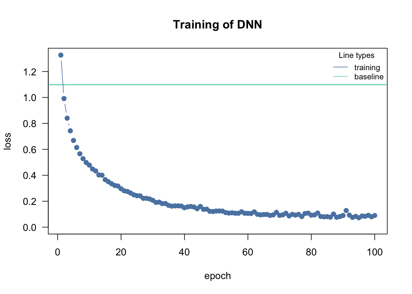
head(predict(model, type = "response")) setosa versicolor virginica
1 0.9972554 0.002744604 9.578507e-11
2 0.9930768 0.006923226 7.367383e-10
3 0.9960633 0.003936661 2.865707e-10
4 0.9920200 0.007980010 1.317580e-09
5 0.9976218 0.002378205 7.866851e-11
6 0.9963681 0.003631910 1.532824e-107.3 Validation split in deep learning
In cito, we can directly tell the dnn function to automatically use a random subset of the data as validation data, which is validated after each epoch (each iteration of the optimization), allowing us to monitor but also to intervene in the training:
data = airquality[complete.cases(airquality),] # DNN cannot handle NAs!
data = scale(data)

model = dnn(Ozone~.,
            validation = 0.2,
            loss = "mse",data = data, verbose = FALSE)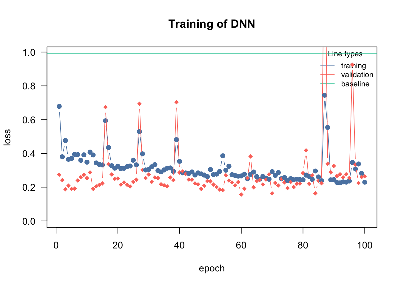
The validation argument ranges from 0 and 1 is the percent of the data that should be used for validation
Warning
The validation split in deep neural networks/ cito is part of the training! It should be not used to validate the model at all. Later on, we will introduce techniques that use the validation data during the training to improve the training itself!
7.3.1 Baseline loss
Since training DNNs can be quite challenging, we provide in cito a baseline loss that is computed from an intercept-only model (e.g., just the mean of the response). And the absolute minimum performance our DNN should achieve is to outperform the baseline model!
7.4 Trainings parameter
In DL, the optimization (the training of the DNN) is challenging as we have to optimize up to millions of parameters (which are not really identifiable, it is accepted that the optimization does not find a global minimum but just a good local minimum). We have a few important hyperparameters that affect only the optimization:
| Hyperparameter | Meaning | Range |
|---|---|---|
| learning rate | the step size of the parameter updating in the iterative optimization routine, if too high, the optimizer will step over good local optima, if too small, the optimizer will be stuck in a bad local optima | [0.00001, 0.5] |
| batch size | NNs are optimized via stochastic gradient descent, i.e. only a batch of the data is used to update the parameters at a time | Depends on the data: 10-250 |
| epoch | the data is fed into the optimization in batches, once the entire data set has been used in the optimization, the epoch is complete (so e.g. n = 100, batch size = 20, it takes 5 steps to complete an epoch) | 100+ (use early stopping) |
7.4.1 Learning rate
cito visualizes the training (see graphic). The reason for this is that the training can easily fail if the learning rate (lr) is poorly chosen. If the lr is too high, the optimizer “jumps” over good local optima, while it gets stuck in local optima if the lr is too small:
model = dnn(Ozone~.,
            hidden = c(10L, 10L),
            activation = c("selu", "selu"),
            loss = "mse", lr = 0.4, data = data, epochs = 150L, verbose = FALSE)
Training curve with a too-high learning rate: the loss is wiggly and may even diverge instead of steadily decreasing.
If too high, the training will either directly fail (because the loss jumps to infinity) or the loss will be very wiggly and doesn’t decrease over the number of epochs.
model = dnn(Ozone~.,
            hidden = c(10L, 10L),
            activation = c("selu", "selu"),
            loss = "mse", lr = 0.0001, data = data, epochs = 150L, verbose = FALSE)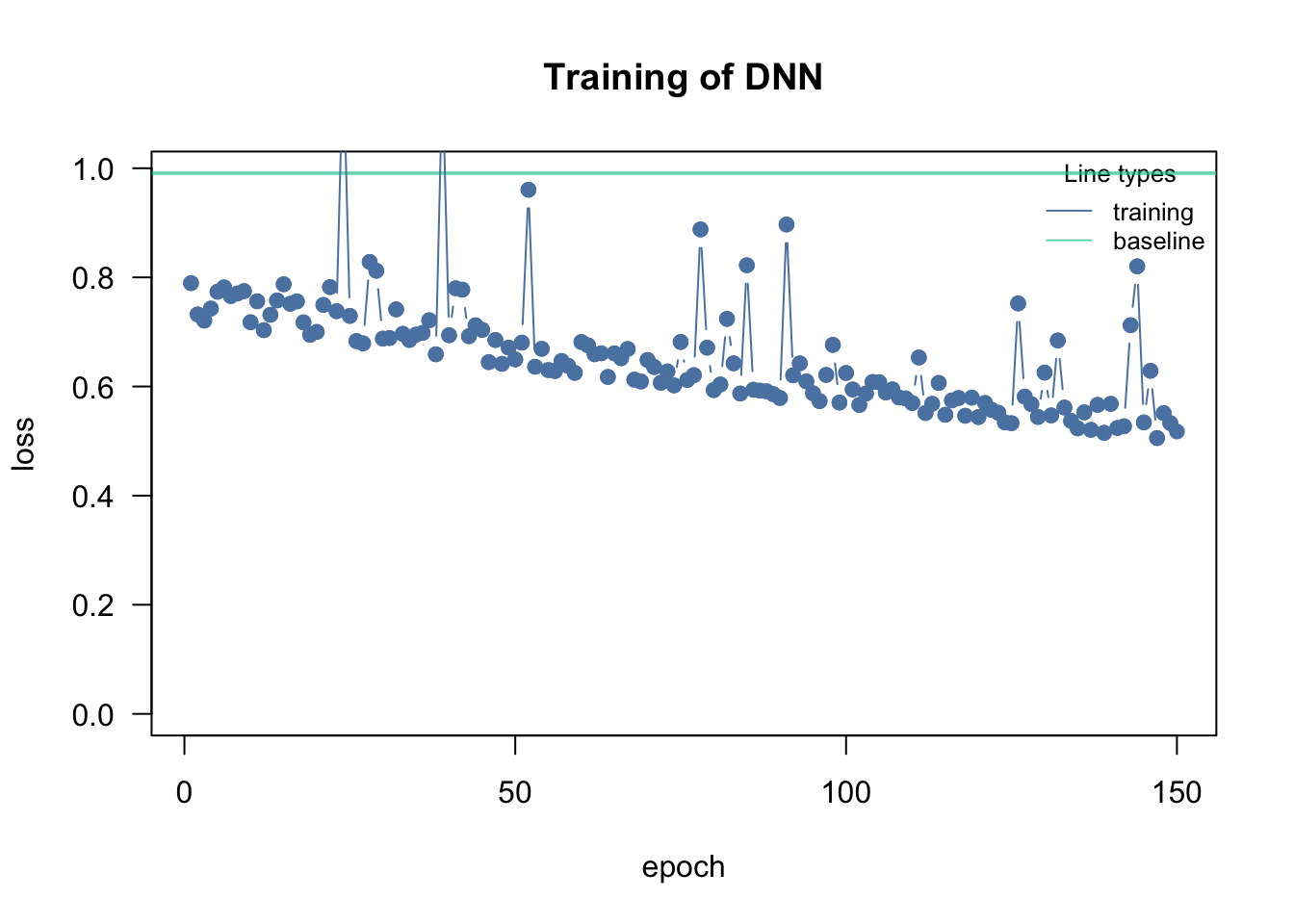
Training curve with a too-low learning rate: the loss decreases only very slowly over the epochs.
If too low, the loss decreases only very slowly over the epochs.
Learning rate scheduler
Adjusting / reducing the learning rate during training is a common approach in neural networks. The idea is to start with a larger learning rate and then steadily decrease it during training (either systematically or based on specific properties):
model = dnn(Ozone~.,
            hidden = c(10L, 10L),
            activation = c("selu", "selu"),
            loss = "mse",
            lr = 0.1,
            lr_scheduler = config_lr_scheduler("step", step_size = 30, gamma = 0.1),
            # reduce learning all 30 epochs (new lr = 0.1* old lr)
            data = data, epochs = 150L, verbose = FALSE)
7.5 Architecture
The architecture of the NN can be specified by the hidden argument, it is a vector where the length corresponds to the number of hidden layers and value of entry to the number of hidden neurons in each layer (and the same applies for the activation argument that specifies the activation functions in the hidden layers). It is hard to make recommendations about the architecture, a kind of general rule is that the width of the hidden layers is more important than the depth of the NN.
Example:
data = airquality[complete.cases(airquality),] # DNN cannot handle NAs!
data = scale(data)

model = dnn(Ozone~.,
            hidden = c(10L, 10L), # Architecture, number of hidden layers and nodes in each layer
            activation = c("selu", "selu"), # activation functions for the specific hidden layer
            loss = "mse", lr = 0.01, data = data, epochs = 150L, verbose = FALSE)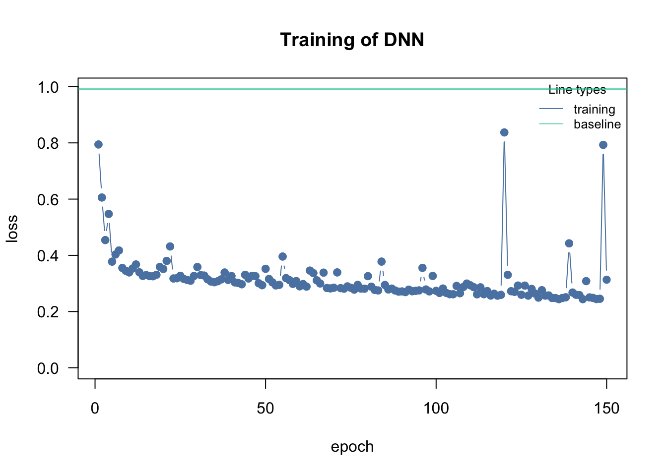
plot(model)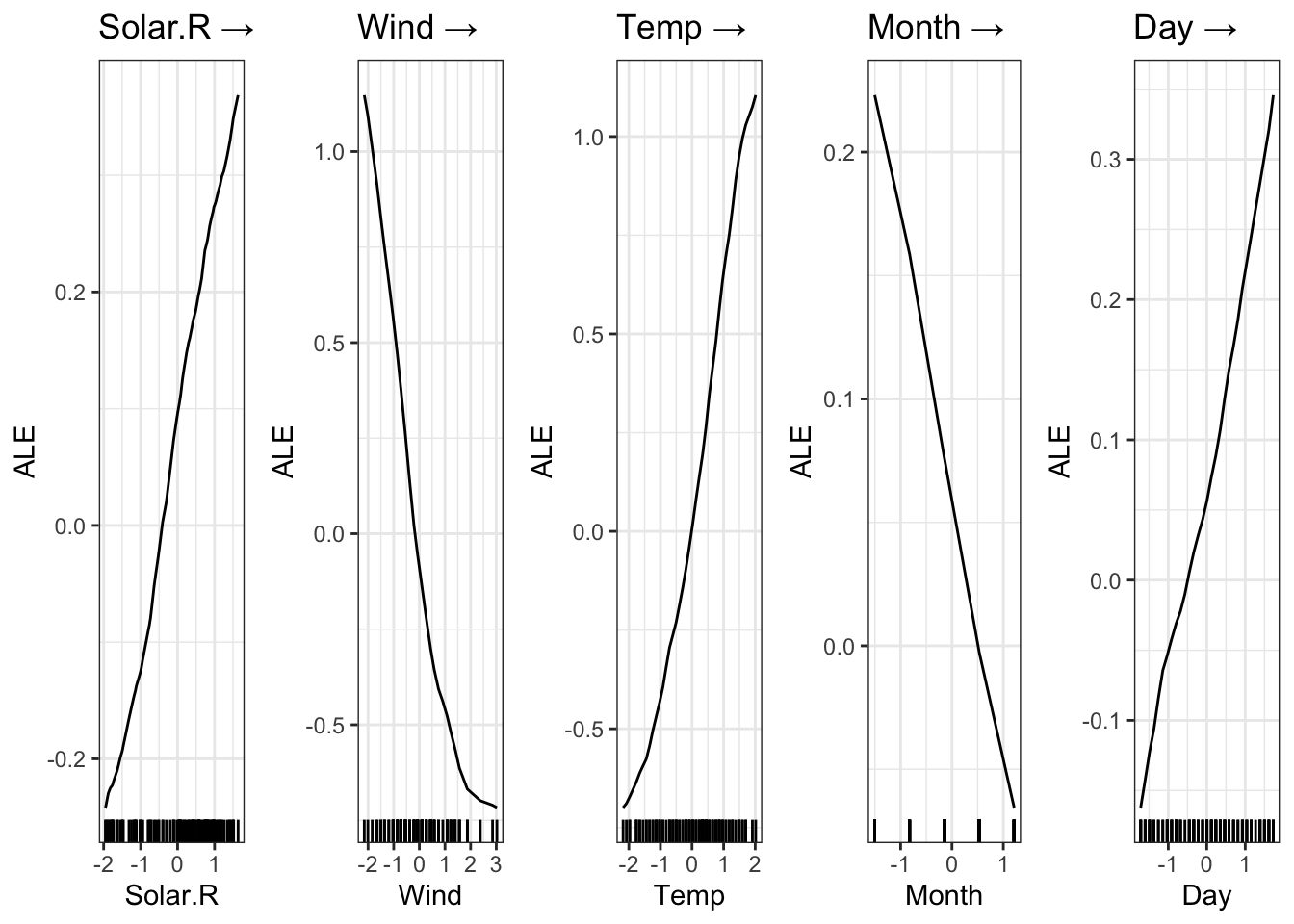
summary(model)Summary of Deep Neural Network Model
Feature Importance:
variable importance_1
1 Solar.R 0.02772261
2 Wind 0.21587175
3 Temp 0.23434401
4 Month 0.01081469
5 Day 0.01716186
Average Conditional Effects:
[,1]
Solar.R 0.16308466
Wind -0.48360296
Temp 0.48883600
Month -0.09708434
Day 0.147884847.6 Regularization
We can use \(\lambda\) and \(\alpha\) to set L1 and L2 regularization on the weights in our NN:
model = dnn(Ozone~.,
            hidden = c(10L, 10L),
            activation = c("selu", "selu"),
            loss = "mse",
            lr = 0.01,
            lambda = 0.01, # regularization strength
            alpha = 0.5,
            lr_scheduler = config_lr_scheduler("step", step_size = 30, gamma = 0.1),
            # reduce learning all 30 epochs (new lr = 0.1* old lr)
            data = data, epochs = 150L, verbose = FALSE)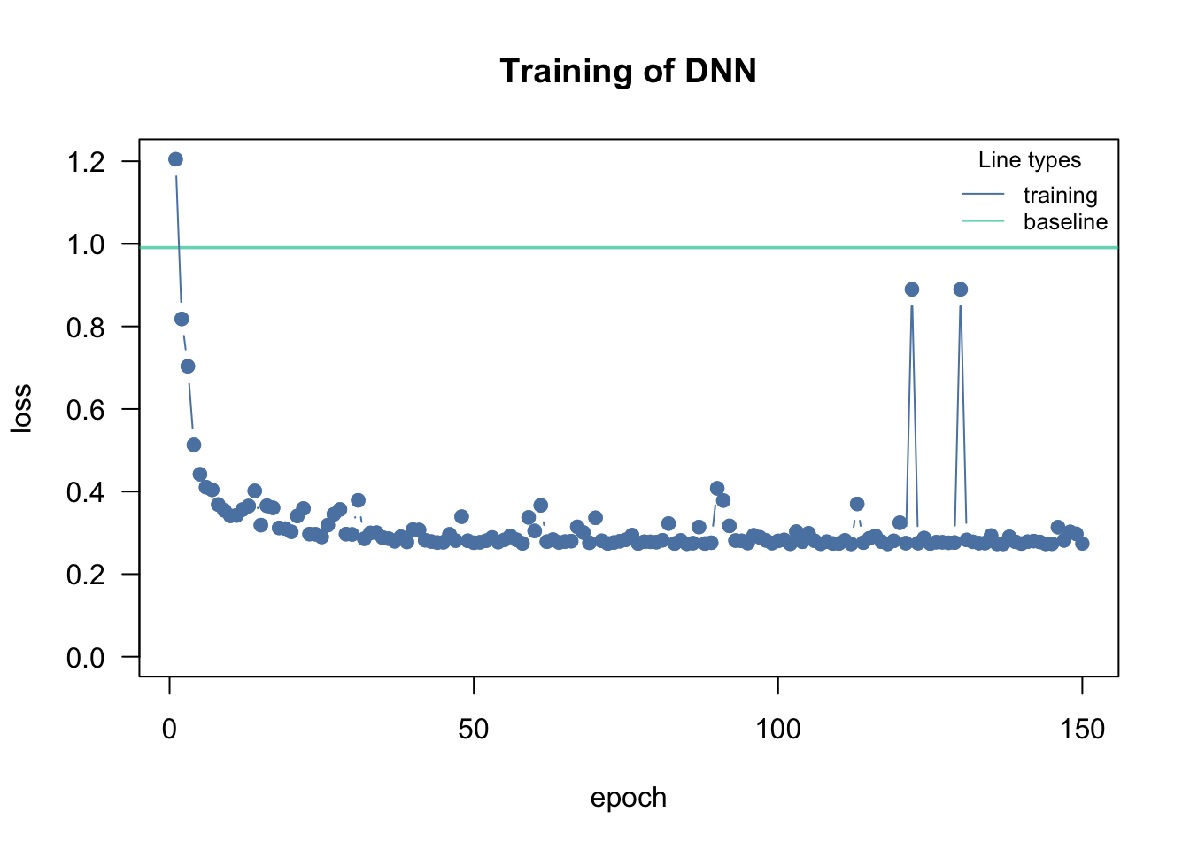
summary(model)Summary of Deep Neural Network Model
Feature Importance:
variable importance_1
1 Solar.R 0.025643307
2 Wind 0.110213420
3 Temp 0.233370949
4 Month 0.009019475
5 Day 0.002193025
Average Conditional Effects:
[,1]
Solar.R 0.17071739
Wind -0.35955328
Temp 0.50049555
Month -0.09378862
Day 0.04677432Be careful that you don’t accidentally set all weights to 0 because of a too high regularization. We check the weights of the first layer:
fields::image.plot(coef(model)[[1]][[1]]) # weights of the first layer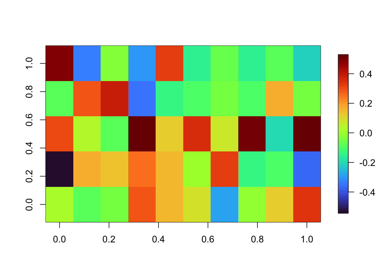
7.7 Hyperparameter tuning
cito has a feature to automatically tune hyperparameters under Cross Validation!
- if you pass the function
tune(...)to a hyperparameter, this hyperparameter will be automatically tuned - in the
tuning = config_tuning(...)argument, you can specify the cross-validation strategy and the number of hyperparameters that should be tested - after the tuning, cito will fit automatically a model with the best hyperparameters on the full data and will return this model
Minimal example with the iris dataset:
df = iris
df[,1:4] = scale(df[,1:4])

model_tuned = dnn(Species~.,
                  loss = "cross-entropy",
                  data = iris,
                  lambda = tune(lower = 0.0, upper = 0.2), # you can pass the "tune" function to a hyerparameter
                  tuning = config_tuning(CV = 3, steps = 20L),
                  verbose = FALSE
                  )
Starting hyperparameter tuning...
Fitting final model...# tuning results
model_tuned$tuning# A tibble: 20 × 5
steps test train models lambda
<int> <dbl> <dbl> <lgl> <dbl>
1 1 104. 0 NA 0.113
2 2 169. 0 NA 0.169
3 3 119. 0 NA 0.134
4 4 117. 0 NA 0.133
5 5 141. 0 NA 0.151
6 6 108. 0 NA 0.118
7 7 19.8 0 NA 0.0114
8 8 75.4 0 NA 0.0887
9 9 14.8 0 NA 0.00745
10 10 73.5 0 NA 0.0862
11 11 74.4 0 NA 0.0743
12 12 168. 0 NA 0.155
13 13 79.0 0 NA 0.116
14 14 33.9 0 NA 0.0233
15 15 169. 0 NA 0.164
16 16 72.7 0 NA 0.0777
17 17 168. 0 NA 0.171
18 18 31.6 0 NA 0.0206
19 19 168. 0 NA 0.161
20 20 73.9 0 NA 0.0789 # model_tuned is now already the best model!7.8 Exercise
7.8.0.1 Tune a DNN — Titanic dataset
Goal: tune a deep neural network on the titanic data and submit your predictions.
Tasks
- Tune the learning rate (
lr) and the regularization (lambdaandalpha). - Interpret: the learning rate is the parameter that most often breaks DNN training. From the loss curve, how can you tell that your learning rate is too high or too low?
Quick check — if the training loss is very wiggly or jumps around instead of decreasing smoothly, the learning rate is most likely:
Hints
In the tree chapter you wrote the cross-validation loop by hand. cito can do the same thing automatically — it tunes hyperparameters under cross-validation for you:
- passing
tune(...)to a hyperparameter will tell cito to tune this specific hyperparameter - the
tuning = config_tuning(...)let you specify the cross-validation strategy and the number of hyperparameters that should be tested (steps = number of hyperparameter combinations that should be tried) - after tuning, cito will fit automatically a model with the best hyperparameters on the full data and will return this model
Minimal example with the iris dataset:
library(cito)
df = iris
df[,1:4] = scale(df[,1:4])
model_tuned = dnn(Species~.,
loss = "cross-entropy",
data = iris,
lambda = tune(lower = 0.0, upper = 0.2), # you can pass the "tune" function to a hyerparameter
tuning = config_tuning(CV = 3, steps = 20L),
burnin = Inf
)
# tuning results
model_tuned$tuning
# model_tuned is now already the best model!library(EcoData)
library(dplyr)
library(missRanger)
data(titanic_ml)
data = titanic_ml
data =
data |> select(survived, sex, age, fare, pclass)
data[,-1] = missRanger(data[,-1], verbose = 0)
data_sub =
data |>
mutate(age = scales::rescale(age, c(0, 1)),
fare = scales::rescale(fare, c(0, 1))) |>
mutate(sex = as.integer(sex) - 1L,
pclass = as.integer(pclass - 1L))
data_new = data_sub[is.na(data_sub$survived),] # for which we want to make predictions at the end
data_obs = data_sub[!is.na(data_sub$survived),] # data with known response
model = dnn(survived~.,
hidden = c(10L, 10L), # change
activation = c("selu", "selu"), # change
loss = "binomial",
lr = 0.05, #change
validation = 0.2,
lambda = 0.001, # change
alpha = 0.1, # change
burnin = Inf,
lr_scheduler = config_lr_scheduler("reduce_on_plateau", patience = 10, factor = 0.9),
data = data_obs, epochs = 40L, verbose = FALSE, plot= TRUE)
# Predictions:
predictions = predict(model, newdata = data_new, type = "response") # change prediction type to response so that cito predicts probabilities
write.csv(data.frame(y = predictions[,1]), file = "Max_titanic_dnn.csv")7.8.0.2 Tune a DNN — Plant-pollinator dataset
The plant-pollinator database is a collection of plant-pollinator interactions with traits for plants and pollinators. The idea is pollinators interact with plants when their traits fit (e.g. the tongue of a bee needs to match the shape of a flower). We explored the advantage of machine learning algorithms over traditional statistical models in predicting species interactions in our paper. If you are interested you can have a look here.
see Section A.3 for more information about the dataset.
Prepare the data:
library(EcoData)
library(dplyr)
Attaching package: 'dplyr'The following objects are masked from 'package:stats':
filter, lagThe following objects are masked from 'package:base':
intersect, setdiff, setequal, uniondata(plantPollinator_df)
plant_poll = plantPollinator_df
summary(plant_poll) crop insect type
Vaccinium_corymbosum: 256 Andrena_wilkella : 80 Length :20480
Brassica_napus : 256 Andrena_barbilabris: 80 N.unique : 2
Carum_carvi : 256 Andrena_cineraria : 80 N.blank : 0
Coriandrum_sativum : 256 Andrena_flavipes : 80 Min.nchar: 9
Daucus_carota : 256 Andrena_gravida : 80 Max.nchar: 10
Malus_domestica : 256 Andrena_haemorrhoa : 80
(Other) :18944 (Other) :20000
season diameter corolla colour
Length :20480 Min. : 2.00 Length :20480 Length :20480
N.unique : 11 1st Qu.: 5.00 N.unique : 3 N.unique : 7
N.blank : 0 Median : 19.00 N.blank : 0 N.blank : 0
Min.nchar: 4 Mean : 27.03 Min.nchar: 4 Min.nchar: 3
Max.nchar: 8 3rd Qu.: 25.00 Max.nchar: 11 Max.nchar: 6
NAs : 1024 Max. :150.00 NAs : 256 NAs : 256
NAs :9472
nectar b.system s.pollination inflorescence
Length :20480 Length :20480 Length :20480 Length :20480
N.unique : 2 N.unique : 4 N.unique : 2 N.unique : 4
N.blank : 0 N.blank : 0 N.blank : 0 N.blank : 0
Min.nchar: 2 Min.nchar: 7 Min.nchar: 2 Min.nchar: 3
Max.nchar: 3 Max.nchar: 13 Max.nchar: 3 Max.nchar: 17
NAs : 1024
composite guild tongue body
Length :20480 Length :20480 Min. : 2.000 Min. : 2.00
N.unique : 2 N.unique : 14 1st Qu.: 4.800 1st Qu.: 8.00
N.blank : 0 N.blank : 0 Median : 6.600 Median :10.50
Min.nchar: 2 Min.nchar: 5 Mean : 8.104 Mean :10.66
Max.nchar: 3 Max.nchar: 14 3rd Qu.:10.500 3rd Qu.:13.00
Max. :26.400 Max. :25.00
NAs :17040 NAs :6160
sociality feeding interaction
Length :20480 Length :20480 0 :14095
N.unique : 2 N.unique : 3 1 : 595
N.blank : 0 N.blank : 0 NAs: 5790
Min.nchar: 2 Min.nchar: 9
Max.nchar: 3 Max.nchar: 11
NAs : 960 NAs : 2160
# scale numeric features
plant_poll[, sapply(plant_poll, is.numeric)] = scale(plant_poll[, sapply(plant_poll, is.numeric)])

# remove NAs
df = plant_poll[complete.cases(plant_poll),] # remove NAs

# remove factors with only one level
data_obs = df |> select(-crop, -insect, -season, -colour, -guild, -feeding, -composite)

# change response to integer (because cito wants integer 0/1 for binomial data)
data_obs$interaction = as.integer(data_obs$interaction) - 1


# prepare the test data
newdata = plant_poll[is.na(plantPollinator_df$interaction), ]
newdata_imputed = missRanger::missRanger(data = newdata[,-ncol(newdata)], verbose = 0) # fill NAs
newdata_imputed$interaction = NA
Minimal example in cito:
data_obs$interaction = as.factor(data_obs$interactions)
library(cito)
set.seed(42)
model = dnn(interaction~.,
    hidden = c(50, 50),
    activation = "selu",
    loss = "binomial",
    lr = tune(values = seq(0.0001, 0.03, length.out = 10)),
    batchsize = 100L, # increasing the batch size will reduce the runtime
    data = data_obs,
    epochs = 200L,
    burnin = Inf,
    tuning = config_tuning(CV = 3, steps = 10))


print(model$tuning)

# make final predictions
predictions = predict(model, newdata_imputed, type = "response")[,1]

# prepare submissions
write.csv(data.frame(y = predictions), file = "my_submission.csv")
7.8.0.3 A note on class imbalance
Before tuning, look at the response:
table(data_obs$interaction)
  0   1
789 107
The data are strongly imbalanced — there are far more non-interactions (0) than interactions (1). This matters for two reasons. First, a model can reach high accuracy simply by predicting “no interaction” every time, so accuracy is a misleading score here; we use the AUC instead, which measures how well the model ranks true interactions above non-interactions regardless of the class sizes. Second, you can optionally rebalance the training data — for example by undersampling the 0s or oversampling the 1s — so the network sees a less skewed mix. Both the loss choice and any rebalancing are modelling decisions worth experimenting with.
Your Tasks:
- Use cito to tune the learning parameters and the regularization (
lr,lambda,alpha). - Submit your predictions to http://132.199.73.15:8500/.
- Interpret: the data are imbalanced. Why do we score this task with the AUC rather than the accuracy, and would balancing the classes change which metric you should trust?
Quick check — on a strongly imbalanced data set, a classifier that always predicts the majority class will have:
Minimal example:
data_obs$interaction = as.factor(data_obs$interaction)

library(cito)
set.seed(42)
model = dnn(interaction~.,
    hidden = c(50, 50),
    activation = "selu",
    loss = "binomial",
    lr = tune(values = seq(0.0001, 0.03, length.out = 10)),
    lambda = tune(values = seq(0.0001, 0.1, length.out = 10)),
    alpha = tune(),
    batchsize = 100L, # increasing the batch size will reduce the runtime
    data = data_obs,
    epochs = 100L,
    burnin = Inf,
    tuning = config_tuning(CV = 3, steps = 15))


print(model$tuning)
Make predictions:
predictions = predict(model, newdata_imputed, type = "response")[,1]

write.csv(data.frame(y = predictions), file = "Max_plant_.csv")
7.8.0.4 Multi-species SDM with cito
Install the development version of cito via
devtools::install_github('citoverse/cito')Minimal example
load("sdm.RData")

library(cito)


trainX = sdm_env$train
testX = sdm_env$test

trainX = missRanger::missRanger(trainX, num.trees = 50L)
testX = missRanger::missRanger(testX, num.trees = 50L)

cols_sel = sapply(trainX, sd) > 0.001

trainXs = scale(trainX)[, cols_sel]
testXs = scale(testX)[, cols_sel]

colnames(trainXs) = stringr::str_remove(colnames(trainXs), "-")
colnames(trainXs) = stringr::str_remove(colnames(trainXs), "-")
colnames(testXs) = colnames(trainXs)

trainXs = trainXs[, - c(1)]
testXs = testXs[, - c(1)]
testXs[is.na(testXs)] = 0.0
Fit the model
library(cito)
m = dnn(X = as.data.frame(trainXs), Y = Y_train, loss = "bernoulli", ce = FALSE, hidden = c(100, 100, 100), lr = 0.01, epochs = 70L,dropout = 0.3, optimizer = config_optimizer("adam", weight_decay = 0.001 ))

probs = predict(m, newdata = (testXs), type = "response")
Prepare the submissions!
write.csv(data.frame(y = as.vector(probs)),
          file = "sdm.csv", row.names = FALSE)